


Figure 1.
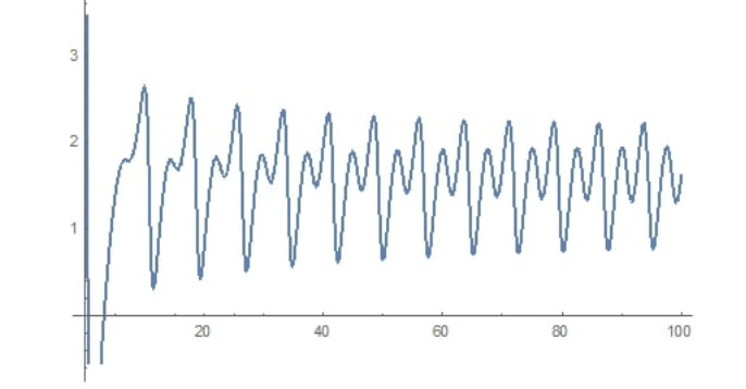
The trajectory of the investment rate x(t), for initial values x(0)=1, y(0)=5, z(0)=1, u(0)=1.
Citation: Eric Ariel L. Salas, Geoffrey M. Henebry. Canopy Height Estimation by Characterizing Waveform LiDAR Geometry Based on Shape-Distance Metric[J]. AIMS Geosciences, 2016, 2(4): 366-390. doi: 10.3934/geosci.2016.4.366
| [1] | John Leventides, Evangelos Melas, Costas Poulios . Extended dynamic mode decomposition for cyclic macroeconomic data. Data Science in Finance and Economics, 2022, 2(2): 117-146. doi: 10.3934/DSFE.2022006 |
| [2] | Aditya Narvekar, Debashis Guha . Bankruptcy prediction using machine learning and an application to the case of the COVID-19 recession. Data Science in Finance and Economics, 2021, 1(2): 180-195. doi: 10.3934/DSFE.2021010 |
| [3] | Georgios Alkis Tsiatsios, John Leventides, Evangelos Melas, Costas Poulios . A bounded rational agent-based model of consumer choice. Data Science in Finance and Economics, 2023, 3(3): 305-323. doi: 10.3934/DSFE.2023018 |
| [4] | Habib Zouaoui, Meryem-Nadjat Naas . Option pricing using deep learning approach based on LSTM-GRU neural networks: Case of London stock exchange. Data Science in Finance and Economics, 2023, 3(3): 267-284. doi: 10.3934/DSFE.2023016 |
| [5] | Ezekiel NN Nortey, Edmund F. Agyemang, Enoch Sakyi-Yeboah, Obu-Amoah Ampomah, Louis Agyekum . AI meets economics: Can deep learning surpass machine learning and traditional statistical models in inflation time series forecasting?. Data Science in Finance and Economics, 2025, 5(2): 136-155. doi: 10.3934/DSFE.2025007 |
| [6] | Manveer Kaur Mangat, Erhard Reschenhofer, Thomas Stark, Christian Zwatz . High-Frequency Trading with Machine Learning Algorithms and Limit Order Book Data. Data Science in Finance and Economics, 2022, 2(4): 437-463. doi: 10.3934/DSFE.2022022 |
| [7] | Ming Li, Ying Li . Research on crude oil price forecasting based on computational intelligence. Data Science in Finance and Economics, 2023, 3(3): 251-266. doi: 10.3934/DSFE.2023015 |
| [8] | Sami Mestiri . Credit scoring using machine learning and deep Learning-Based models. Data Science in Finance and Economics, 2024, 4(2): 236-248. doi: 10.3934/DSFE.2024009 |
| [9] | Man-Fai Leung, Abdullah Jawaid, Sai-Wang Ip, Chun-Hei Kwok, Shing Yan . A portfolio recommendation system based on machine learning and big data analytics. Data Science in Finance and Economics, 2023, 3(2): 152-165. doi: 10.3934/DSFE.2023009 |
| [10] | Lindani Dube, Tanja Verster . Enhancing classification performance in imbalanced datasets: A comparative analysis of machine learning models. Data Science in Finance and Economics, 2023, 3(4): 354-379. doi: 10.3934/DSFE.2023021 |
Chaotic dynamical systems are deterministic dynamical systems which are characterized by the fact that small changes in the initial conditions lead to very large differences at a later time. Chaotic dynamical systems are to be contradistinguished with stochastic dynamical systems. Stochastic dynamical systems are not deterministic and a probability space is required to study their evolution.
In recent years, chaotic systems have been receiving more and more attention and interest because of their potential applications in many areas which range from physics and telecommunications to biological networks and economic models. Since the chaotic phenomenon in economics was discovered in 1985, it has been widely accepted that the economy and the finance systems are very complicated nonlinear systems containing many complex factors and accordingly, many efforts have been devoted to their study (Chian et al., 2006; Gao and Ma, 2009; Gu´egan, 2009; Wijeratne et al., 2009). As stated in chian, characterization of the complex dynamics of economic systems is a powerful tool for pattern recognition and forecasting of business and financial cycles, as well as for optimization of management strategy and decision technology. Therefore, the need for analysis and control of these systems is emerging and many researchers have been working towards this direction.
In this paper, we indicate a method for approximating a macroeconomic chaotic system and reconstructing its trajectories using a linear finite dimensional dynamical system. This method sits across Koopman operators, EDMD, Takens theorem and Machine Learning. EDMD and its precursor DMD, as well as, Koopman operators, Takens' theorem and Machine Learning have been extensively used in Finance (for instance, Hua et al., 2017; Mauroy et al., 2020; Mann and Kutz, 2016; Stavroglou et al., 2019; Ni et al., 2021).
Roughly speaking, the Koopman operator "lifts" the dynamics of the original system from the state space to linear spaces consisting of functions defined on the state space (which are called observables). The advantage of this lifting is that we obtain a linearization of the original system which holds to the whole state space and many properties of the dynamics correspond to spectral properties of the Koopman operator. The disadvantage is that the linear system induced by the Koopman operator is infinite dimensional. Therefore, its dynamics and spectral properties cannot be calculated while several methods for analysis and control cannot be applied.
The Extended Dynamic Mode Decomposition provides us with a method for obtaining finite dimensional approximations of the Koopman operator. These approximations, under some suitable assumptions, converge to the Koopman operator. Therefore, they can also be used to reconstruct the trajectories in the phase space of the original nonlinear system.
The success of EDMD depends on a set of observables (a dictionary) which is chosen a priori. This method is purely data-driven and is based on instantaneous measurements of the values of the observables. Then, the linear dynamical system that is provided advances the measurements form one time to the next.
On the other hand, it is generally feasible to extract information about features of phase space from time series of general measurements made on an evolving system (Sauer et al., 1991). The central result in this direction was proved by (Takens, 1981) who showed how a time series of measurements of a single observable can be used to reconstruct qualitative features of the phase space of the system. The technique described by Takens, the method of delays, is so simple that it can be applied to essentially any time series whatever, and has made possible the wide−ranging search for chaos in dynamical systems. Takens' theorem asserts that the phase space of a dynamical system and in particular strange attractors of the system can be diffeomorphically embedded in a higher dimensional space spanned by an appropriate number of time lags of a single observable of the system.
This is a very powerful result since it allows to recover the dynamics from the observation of just one variable, the embedding preserves the topology of the phase space and it preserves the topology of the attractor in particular, the embedding being a diffeomorphism allows system identification, it also allows to calculate the box-counting dimension of the attractor, and it allows to calculate the (positive) Lyapunov exponents. However, Takens' theorem does not allow reconstruction of the trajectories of the dynamical system. This is to be juxtaposed with the Koopman-EDMD theory which aims at reconstructing the trajectories of the system.
What the two approaches have in common is that both are data-driven since the observables they use are constructed from data measured during the evolution of the system. In Takens' theorem the observables are simpler in form and they are the time lags of a single observable. In Koopman-EDMD theory the observables are usually the state variables of the dynamical system and non−linear functions of them. In this paper we use an hybrid method in order to reconstruct with simple means trajectories of a macroeconomic dynamical system which exhibits chaotic behaviour. In particular we use Koopman-EDMD theory with observables those used by Takens' Theorem. The finite dimensional approximation to the Koopman operator which drives the dynamics and reconstructs the trajectories of the system is obtained by two different methods: By a Linear autoregressive model and by an Autoregression with machine learning methods. The use of the Linear autoregressive model leads to more faithful reconstruction of the trajectories of the dynamical system at hand than the use of Autoregression with machine learning methods. However, this is attributed to the fact the error made in the case of the Linear autoregressive model can be corrected whereas this is not feasible in the case of Autoregression with machine learning methods where the error made in the prediction of the future value of the observable from the previous values cannot be corrected and accumulates over time.
Therefore, the motivation, innovation and contribution of this paper can be summarized as follows: This paper addresses the trajectory approximation of an hyperchaotic system via EDMD methods. The EDMD methods give rise to a linear system on an enhanced state space that can approximate a given trajectory. Having data of a given trajectory in a finite horizon allows to construct a discrete linear system of dimension n>>m, where m is the dimension of the state space of the nonlinear system. Takens' Theorem indicates how large n can be. Here we demonstrate the approximation of a single trajectory of a chaotic system via EDMD methods equivalent to linear Autoregressive construction. Furthermore, we demonstrate the use of the same method on multiple trajectories. Finally, we demonstrate how we can use the same data in order to construct nonlinear trajectory approximation via machine learning methods.
Trajectory approximation of chaotic nonlinear systems is a particularly difficult problem as these trajectories are sensitive to initial conditions and also exhibit variable spectrum and almost periodicity properties. Simultaneous approximation of orbits that differ seems a challenge via any method requiring big data and accurate approaches. The use of linear dynamic models seems in certain respects more appropriate as the knowledge of its structure allows to correct the fitted model if significant part of the spectrum of the data is lost due to numerical or other errors. This is demonstrated in this paper. The conclusions in this paper are derived with the use of an economic model (Yu et al., 2012) which exhibits hyperchaotic behaviour. We note that the scope the methods and the results in this paper are entirely different from those in Yu. In a nutshell in this paper we approximate the trajectory of the hyperchaotic system introduced in Yu via EDMD methods whereas in Yu the general structure of this system is studied, namely, its equilibrium points, its bifurcations, e.t.c..
The EDMD method is data driven. Consequently our method can be applied to any dynamical system for which probably the dynamical law which drives its dynamics is unknown and data, in the form of time series, can be collected for some of its trajectories in state space. Moreover, our approach can be advocated for any nonlinear dynamical system whose dynamical law which drives its dynamics might be known but a linearization of its dynamics via the EDMD method may be required in order for example to study control theory of this linearized system; control theory of linear systems is much better understood than the control theory of nonlinear systems.
The rest of the paper is organized as follows. In Section 2, we firstly review a dynamical system which has emerged from financial studies and it shows chaotic behaviour for some values of the parameters. Furthermore, we briefly present some basic facts about the Koopman operator. We also describe the EDMD algorithm and the main idea about the connections with Takens' theorem. The latter is analyzed with more details in Subsection 2.5. In Section 3 we consider the chaotic system of Section 2.1 and we developed our methodology for approximating and reconstructing a single trajectory of the system. In Section 4, we demonstrate the proposed approach in the case where we wish to simultaneously approximate two orbits of the original system with the same autoregressive model. Finally, Section 5 concludes the paper.
Various financial system have been found to exhibit chaotic dynamics (Chian, 2000; Fanti and Manfredi, 2007; Gu´egan, 2009; Hass, 1998; Holyst et al., 1996; Lorenz, 1993). A lot of research has been invested in the analysis, control and stabilization of these systems (for instance, see Ahmad et al., 2021; Chen et al., 2021; Ma et al., 2022; Pan and Wu, 2022; for some recent studies). In the present paper, we use in our analysis a chaotic dynamical model that describes the time evolution of three state variables: x is the interest rate, y is the investment demand and z is the price exponent. For more details about the origination, the development and the economic interpretation of the model, we refer to ma, Yu, jiang and zhao. The system is described by the following non-linear differential equations.
| {˙x=z+(y−a)x˙y=1−by−x2˙z=−x−cz | (1) |
where a, b, c are positive constant parameters that represent the amount of savings, the cost per investment and the elasticity of demand respectively (see Ma and Chen, 2001).
When the values of parameters are chosen as a=0.9, b=0.2, c=1.2 and for initial conditions (x0,y0,z0)=(1,3,2) the system (1) has a strange attractor that can be classified neither as a stable equilibrium nor as a periodic or almost periodic oscillation. Therefore, the system exhibits chaotic behaviour (see Ma and Chen, 2001; Rigatos, 2017).
Later, in Yu, it was observed that x depends not only on the investment demand and the price exponent, but also on the average profit margin (denoted by u(t)). Therefore, in Yu a dynamical system consisting of four state variables (x,y,z,u) is proposed which is described by the next first order non-linear differential equations
| {˙x=z+(y−a)x+u˙y=1−by−x2˙z=−x−cz˙u=−dxy−ku |
where a,b,c,d,k are positive parameters. It is shown that, if the parameters' values are chosen to be a=0.9, b=0.2, c=1.5, d=0.2, k=0.17, then the system shows hyperchaotic behaviour (see Yu et al., 2012). A hyperchaotic system is usually defined as a chaotic system with more than one positive Lyapunov exponent. Therefore, these system show more complex behaviour than chaotic systems.
The Koopman operator theory represents an increasingly popular formalism of dynamical systems since it allows the analysis of nonlinear and complicated systems. Therefore, it can be utilized in chaotic and hyperchaotic systems.
Assume that (M,f) is a continuous dynamical system, where M⊆Rn is a real manifold, f is the evolution map and the system is described by the equation ˙x=f(x). We also denote by Φt(x0) the flow map defined as the state of the system at time t when we start from the initial condition x0.
Any function g:M→C is called an observable of the system (M,f). Let now F be a function space of observables which enjoys the property: for any g∈F and any t≥0, it holds that g∘Φt∈F. Then, the Koopman operator, which is actually a semigroup of operators, is defined for any t≥0, as Kt:F→F with
| Kt(g)=g∘Φt. |
It is easily verified that Kt is linear for any t≥0. Throughout this paper, following the common practice, we will use the term Koopman operator to refer to the whole class of operators K=(Kt)t≥0. In many applications, the space F coincides with the Hilbert space L2(M), however other choices can be used as well.
Similarly, the Koopman operator can be defined for any discrete dynamical system xk+1=f(xk) defined on the state space M. The Koopman operator is the composition of any observable with the evolution map f, that is, K:F→F is defined by K(g)=g∘f, for any observable g∈F. Here, F is a linear space of observables which is closed under composition with f and the space L2(M) remains a standard choice.
Roughly speaking the Koopman operator updates every observable in the space F according to the evolution of the dynamical system. It defines a linear dynamical system (F,K) which completely describes the original system (M,f). This linearization is applied to any nonlinear system and it is global, i.e. it does not hold only to the area of some attractor or fixed point. Furthermore, many properties of the original system can be codified as properties of the Koopman operator and, usually they can be related to the eigenstructure of K. However, since K is usually infinite dimensional, its spectral properties cannot be calculated except some rare cases.
To overcome the problem of dimensionality, one has to look for finite dimensional approximations of the Koopman operator, i.e. finite dimensional subspaces of the domain of K which are invariant under K. The most natural candidates for this project are the spaces generated by eigenvectors of K, which, however, are difficult to find. Hence, we are obliged to search for finite dimensional linear approximations of the Koopman operator. Towards this direction, the Dynamic Mode Decomposition (DMD) and its generalization the so-called Extended Dynamic Mode Decomposition (EDMD) have been proved very successful.
We next describe briefly the main steps of the EDMD algorithm. Firstly, one has to consider a set of observables {g1,g2,…,gp}. This set is usually called a dictionary. The cardinality p of the dictionary is expected to be much bigger than n (the dimension of the original state space M). The DMD (Dynamic Mode Decomposition) uses only the observables gi(x)=xi, for i=1,2,…,n. However, in EDMD we can choose any observables. Hence, an augmented state space is constructed and EDMD provides, in general, better approximations than DMD. We denote the augmented state space by ¯M and its elements by y=[g1(x),…,gp(x)]T.
The second step is to collect the data. We consider a trajectory of the original system with initial condition x0. The trajectory is witnessed for some finite time horizon T and sampling points are collected at a fixed time interval ΔT. Uniform sampling is not mandatory and other sampling methods can be applied. Therefore, n0=TΔT points in this trajectory are considered. We denote our data by
| (xs)n0s=0. |
These data correspond to data (ys)n0s=0 in the augmented space ¯M. We now consider the data matrices
| Y[0,n0−1]=[y0,y1,…,yn0−1]andY[1,n0]=[y1,y2,…,yn0]. |
Finally, using least square regression methods, we obtain a p×p matrix A, such that Y[1,n0]∼AY[0,n0−1]. Therefore, we have
| A=argmin˜A∈Rp×p‖Y[1,n0]−˜AY[0,n0−1]‖. |
Here, ‖⋅‖ denotes some matrix norm, for instance the Frobenius norm.
This procedure can also be applied to several trajectories. In this case, we construct data matrices Yj[0,n0−1] and Yj[01,n0] for every trajectory j=1,2,…,k. Then, the matrix A is chosen such that
| A=argmin˜A∈Rp×pk∑j=1‖Yj[1,n0]−˜AYj[0,n0−1]‖. |
Roughly speaking, A is a best-fit matrix which relates the two data matrices in every trajectory. This matrix generates a finite dimensional linear system that advances spatial measurements from one time to the next and therefore it may provide approximations of the original nonlinear system.
One of the advantages of the EDMD method is that it depends on data. Hence, it may be applied when the dynamics of the system is unknown. On the other hand, the success of this method depends on the dictionary which is chosen a priori. In many cases, it is a difficult problem to find the suitable observables. Recent studies try to utilize machine learning and artificial intelligence methods in order to "train" the dictionary.
As it has been mentioned, EDMD advances measurements of the state of the system from one time to the next. However, we may also obtain measurements coordinates for the approximation of Koopman operator using time-delayed measurements of the system. This approach is also data-driven and utilize the information from the previous measurements to predict the future. It is particularly useful in chaotic systems. In the case of fixed points or periodic orbits, more data from previous measurements have small contributions. On the contrary, when the trajectories densely fill a strange attractor, more data provide more information.
From this point of view, Koopman operators can interact with Takens embedding theorem. The latter could provide us information about the dimensions of the augmented state-space as well as the dictionary that should be chosen. A connection between Koopman operators and Takens Theorem has already been investigated in bana.
We firstly need some definitions. A dynamical system on a manifold M is specified by a flow
| ϕ(⋅)(⋅):R×M→M, |
where ϕ0(x)=x, ϕt is a diffeomorphism for all t and ϕt∘ϕs=ϕt+s (e.g. ϕ is the solution to a system of ODEs).
Roughly speaking, an attractor of a dynamical system is a subset of the state space to which orbits originating from typical initial conditions tend as time increases. It is very common for dynamical systems to have more than one attractor. For each such attractor, its basin of attraction is the set of initial conditions leading to long−time behavior that approaches that attractor.
An attracting set A for the flow ϕt is a closed set such that:
● the basin of attraction B(A) has positive measure,
● for A′⊆A the difference B(A)∖B(A′) has positive measure.
A set A⊂M is an attractor if it is an attracting set that contains a dense orbit of the flow ϕt. An attractor A is strange attractor ((Eckmann and Ruelle, 1985; Guckenheimer and Holmes, 1983), if its box-counting dimension d is non-integer.
Theorem 2.1 (Takens' theorem). Let M be a compact manifold of (integer) dimension q. Then for generic pairs (ϕ,y), where
● ϕ:M→M is a C2−diffeomorphism of M in itself,
● y:M→M is a a C2−differentiable function,
the map Φ(ϕ,y):M→R2q+1 given by
| Φ(ϕ,y)(x):=(y(x),y(ϕ(x)),y(ϕ2(x)),...,y(ϕ2q(x))) |
is an embedding (i.e. an injective and an immersive map) of M in R2q+1.
If ϕt is a flow on M and τ>0 is a fixed time, then we can define the delay map by
| Φ(x):=(y(x),y(ϕ−τ(x)),y(ϕ−2τ(x)),...,y(ϕ−κτ(x))). | (2) |
If M is a manifold that is an attractor for the flow ϕt, then ϕ−τ is a diffeomorphism of M into itself, so if κ≥2dim(M)+1 for generic y,τ, Takens' theorem (see Sauer et al., 1991; Packard et al., 1980; Takens, 1981; Muldoon et al., 1993) says that the delay map defined by (2) is actually an embedding.
Finally, we close with some details about the meaning of generic. Let P be a property of functions in Ck(M,N) they might or might not have. Then we say that P(f) is true for generic f∈Ck(M,N) if the set of functions for which it holds is open and dense in the Ck topology. So arbitrary small perturbations turn bad choices in good choices.
The central plank of this theory is a result− suggested by several people (Packard et al., 1980) and eventually proved in (Takens, 1981)− which shows how a time series of measurements of a single observable can often be used to reconstruct qualitative features of the phase space of the system. The technique described by Takens, the method of delays (2), is so simple that it can be applied to essentially any time series whatever, and has made possible the wide-ranging search for chaos.
We consider the 4-dimensional (financial) dynamical system described in Section 2.1, which for the parameter values a=0.9, b=0.2, c=1.5, d=0.2, k=0.17 exhibits chaotic behaviour. We select initial conditions for the four variables to be: x(0)=1, y(0)=5, z(0)=1, u(0)=1. For this values the trajectory for x(t) is depicted in Figure 1.
The vector of variables (x,y,z,u) converges to a chaotic attractor in R4. According to Whitney Takens theorem we can embed this attractor to a higher dimensional space of dimension d at least 8 by considering a single observable and a vector of d of its lagged values. We try to use this idea so that to attempt to reconstruct the above trajectory by using a 9-dimensional dynamical system. The simplest way to do that is to consider x as an observable and to model the evolution of the vector (x(T−9Δt),…,x(T)) assuming a sampling period Δt in our case Δt=1.
The simplest model for this evolution is a linear autoregressive model
| xn+9=a8xn+8+…+a0xn. |
We model the time series of the above plotted variable x(t) obtained after sampling and we get the results showed in Tables 1 and 2. Using these results, we reconstruct the x trajectory as shown in Figure 2.
| Estimate | Standard error | t-Statistic | p-value | |
| ♯1 | 0.382345 | 0.0526912 | 7.25634 | 1.1104 ×10⁻¹¹ |
| ♯2 | 0.0528833 | 0.0593214 | 0.891471 | 0.373854 |
| ♯3 | 0.0510388 | 0.0532897 | 0.95776 | 0.339454 |
| ♯4 | 0.0669098 | 0.0533061 | 1.2552 | 0.211016 |
| ♯5 | −0.0546443 | 0.0532567 | −1.02606 | 0.306227 |
| ♯6 | −0.0756992 | 0.0534338 | −1.41669 | 0.158283 |
| ♯7 | 0.488672 | 0.0536388 | 9.11044 | 1.47733 ×10⁻¹⁶ |
| ♯8 | 0.457925 | 0.0622202 | 7.35974 | 6.12628 ×10⁻¹² |
| ♯9 | −0.374469 | 0.040841 | −9.16895 | 1.01965 ×10⁻¹⁶ |
 DownLoad:
CSV
DownLoad:
CSV
| DF | SS | MS | F-Statistic | p-value | |
| ♯1 | 1 | 440.283 | 440.283 | 12718.8 | 2.36926 ×10−170 |
| ♯2 | 1 | 0.252312 | 0.252312 | 7.28877 | 0.00759293 |
| ♯3 | 1 | 39.9561 | 39.9561 | 1154.25 | 1.03165 ×10−80 |
| ♯4 | 1 | 0.388756 | 0.388756 | 11.2304 | 0.000978538 |
| ♯5 | 1 | 0.447058 | 0.447058 | 12.9146 | 0.000419584 |
| ♯6 | 1 | 4.09436 | 4.09436 | 118.277 | 1.52056 ×10⁻²¹ |
| ♯7 | 1 | 9.81632 | 9.81632 | 283.573 | 5.71589 ×10−39 |
| ♯8 | 1 | 0.0967607 | 0.0967607 | 2.79521 | 0.0962645 |
| ♯9 | 1 | 2.9102 | 2.9102 | 84.0696 | 1.01965 ×10⁻¹⁶ |
| Error | 182 | 6.30022 | 0.0346166 | ||
| Total | 191 | 504.545 |
DownLoad:
CSV

Furthermore, we extrapolate the modes of the above AR system which have modulus close to unity on the unit circle by radial projection. The new AR system reconstructs x(t) as depicted in Figure 3.

The above results demonstrate that the considered chaotic financial system can be approximated, at least orbitwise and in finite horizon, by AR models of high enough dimensions and thus EDMD methods may assist in modeling the Takens embedding for the purpose of simulating single or multiple chaotic trajectories.
Finally, we apply two further methods to explore nonlinear relationships for the transition proposed by the Takens embedding using machine learning methods. Both are generally described by a nonlinear autoregression
| xn+9=F(xn+8,…,xn), |
which was realised by two machine learning approaches, namely random forest interpolation and Gaussian process interpolation. The results for the same trajectory reconstruction are depicted in Figures 4 (for random forests) and 5 (for Gaussian process interpolation). Details of the two approaches are given in Tables 3 and 4.

| Predictor information | |
| Method | Random Forest |
| Number of features | 1 |
| Number of training examples | 190 |
| Number of trees | 50 |
DownLoad:
CSV
| Predictor information | |
| Method | Gaussian process |
| Number of features | 1 |
| Number of training examples | 190 |
| Assume Deterministic | False |
| Numerical Covariance Type | Squared Exponential |
| Nominal Covariance Type | Hamming Distance |
| Estimation Method | Maximum Posterior |
| Optimization Method | Find Minimum |
DownLoad:
CSV
Both methods fit well to the training data however when used for trajectory reconstruction starting from the same initial condition the subsequent calculation of the trajectory suffers from error accumulation and therefore reconstruction worsens with time. Gaussian process interpolation seems to work better.
In this section, we try to simultaneously approximate two orbits of the hyperchaotic dynamical system via a single autoregressive dynamical system. To achieve this goal we need to increase the number of lags to 30.
First of all, we use data from numerical integration to plot the second orbit. This orbit is shown in Figure 6 and corresponds to initial conditions x(0)=0, y(0)=2, z(0)=0 and u(0)=1 and time horizon t∈[0,100]. We note that the new initial conditions give rise to an orbit that is quite far from the first one. Hence, the task of the simultaneous approximation is quite challenging. The new autoregression is supposed to produce a new dynamical system that approximate the two trajectories by a single autoregressive equation and different initial conditions.


Similarly to the case of one trajectory, the simplest autoregressive model that one may consider is linear. The regression results are depicted in Table 6. The value of the adjusted R2 is 0.9777954946531674. We can see that this value is smaller than the corresponding value of the one orbit case, however, it is still very close to 1. The regression function is given by:
| xn+31=30∑j=1ajxn+j, |
| DF | SS | MS | F-Statistic | p-value | |
| ♯1 | 1 | 885.406 | 885.406 | 13286.5 | 1.38351 ×10−256 |
| ♯2 | 1 | 0.466206 | 0.466206 | 6.99591 | 0.00858584 |
| ♯3 | 1 | 24.5391 | 24.5391 | 368.235 | 1.2149 ×10−54 |
| ♯4 | 1 | 1.85537 | 1.85537 | 27.8417 | 2.47799 ×10⁻⁷ |
| ♯5 | 1 | 2.68491 | 2.68491 | 40.2899 | 7.76562 ×10⁻¹⁰ |
| ♯6 | 1 | 17.6117 | 17.6117 | 264.283 | 2.08632 ×10−43 |
| ♯7 | 1 | 23.8109 | 23.8109 | 357.307 | 1.51675 ×10−53 |
| ♯8 | 1 | 11.7662 | 11.7662 | 176.565 | 3.37191 ×10⁻³² |
| ♯9 | 1 | 6.70749 | 6.70749 | 100.653 | 1.07024 ×10⁻²⁰ |
| ♯10 | 1 | 0.204543 | 0.204543 | 3.06939 | 0.0807683 |
| ♯11 | 1 | 8.20769 | 8.20769 | 123.165 | 2.54294 ×10⁻²⁴ |
| ♯12 | 1 | 0.0414977 | 0.0414977 | 0.622716 | 0.430643 |
| ♯13 | 1 | 0.0341088 | 0.0341088 | 0.511839 | 0.474883 |
| ♯14 | 1 | 1.21188 | 1.21188 | 18.1856 | 0.0000266385 |
| ♯15 | 1 | 2.18295 | 2.18295 | 32.7575 | 2.46335 ×10⁻⁸ |
| ♯16 | 1 | 1.68824 | 1.68824 | 25.3338 | 8.1894 ×10⁻⁷ |
| ♯17 | 1 | 0.371216 | 0.371216 | 5.57049 | 0.0188848 |
| ♯18 | 1 | 4.50535 | 4.50535 | 67.6076 | 5.53381 ×10⁻¹⁵ |
| ♯19 | 1 | 0.313024 | 0.313024 | 4.69725 | 0.030972 |
| ♯20 | 1 | 0.360659 | 0.360659 | 5.41207 | 0.0206423 |
| ♯21 | 1 | 0.718296 | 0.718296 | 10.7788 | 0.00114403 |
| ♯22 | 1 | 1.03007 | 1.03007 | 15.4573 | 0.000104143 |
| ♯23 | 1 | 1.23863 | 1.23863 | 18.5869 | 0.0000218361 |
| ♯24 | 1 | 0.0496161 | 0.0496161 | 0.744542 | 0.388877 |
| ♯25 | 1 | 0.00615967 | 0.00615967 | 0.0924324 | 0.761311 |
| ♯26 | 1 | 0.202932 | 0.202932 | 3.0452 | 0.0819668 |
| ♯27 | 1 | 2.1012 | 2.1012 | 31.5307 | 4.36478 ×10⁻⁸ |
| ♯28 | 1 | 0.157497 | 0.157497 | 2.36341 | 0.125231 |
| ♯29 | 1 | 0.199552 | 0.199552 | 2.99448 | 0.0845438 |
| ♯30 | 1 | 0.0705909 | 0.0705909 | 1.05929 | 0.304179 |
| Error | 310 | 20.6583 | 0.0666397 | ||
| Total | 340 | 1020.4 |
DownLoad:
CSV
| Estimate | Standard error | t-Statistic | p-value | |
| ♯1 | 0.245794 | 0.0552653 | 4.44753 | 0.0000121198 |
| ♯2 | −0.473285 | 0.0566816 | −8.34989 | 2.30183 ×10⁻¹⁵ |
| ♯3 | −0.00730259 | 0.0626806 | −0.116505 | 0.907368 |
| ♯4 | −0.384589 | 0.0599047 | −6.42001 | 5.1073 ×10⁻¹⁰ |
| ♯5 | −0.244072 | 0.0613891 | −3.97582 | 0.0000873291 |
| ♯6 | 0.353163 | 0.0626402 | -5.63797 | 3.87278 ×10⁻⁸ |
| ♯7 | 0.00100867 | 0.0631682 | 0.0159681 | 0.98727 |
| ♯8 | −0.142987 | 0.0620628 | −2.30391 | 0.0218891 |
| ♯9 | 0.136853 | 0.0610078 | 2.24321 | 0.0255892 |
| ♯10 | −0.241157 | 0.0608958 | −3.96016 | 0.0000929613 |
| ♯11 | 0.167892 | 0.0599006 | 2.80285 | 0.00538436 |
| ♯12 | −0.128651 | 0.0605339 | -−2.12527 | 0.0343548 |
| ♯13 | 0.0686504 | 0.0554803 | 1.23738 | 0.216881 |
| ♯14 | −0.0330885 | 0.0555248 | −0.595923 | 0.551661 |
| ♯15 | 0.327951 | 0.0537379 | 6.10279 | 3.10786 ×10⁻⁹ |
| ♯16 | −0.0368829 | 0.0559783 | −0.658877 | 0.510464 |
| ♯17 | 0.171794 | 0.0557006 | 3.08425 | 0.00222441 |
| ♯18 | 0.357909 | 0.0566593 | 6.31687 | 9.25464 ×10⁻¹⁰ |
| ♯19 | 0.194009 | 0.0603826 | 3.213 | 0.00145176 |
| ♯20 | 0.0956424 | 0.0602179 | 1.58827 | 0.113244 |
| ♯21 | 0.247097 | 0.0593144 | 4.16589 | 0.0000402579 |
| ♯22 | 0.183056 | 0.0604346 | 3.029 | 0.00265998 |
| ♯23 | 0.335842 | 0.060323 | 5.5674 | 5.60543 ×10⁻⁸ |
| ♯24 | −0.00644882 | 0.0597654 | −0.107902 | 0.914143 |
| ♯25 | 0.162157 | 0.0582993 | 2.78146 | 0.00574279 |
| ♯26 | −0.102138 | 0.0573372 | −1.78136 | 0.0758319 |
| ♯27 | 0.301513 | 0.0564203 | 5.34406 | 1.76445 ×10⁻⁷ |
| ♯28 | 0.0609255 | 0.0545446 | 1.11699 | 0.264865 |
| ♯29 | 0.0523586 | 0.0520694 | 1.00555 | 0.315414 |
| ♯30 | 0.0408878 | 0.039727 | 1.02922 | 0.304179 |
DownLoad:
CSV
where (aj)3j=10 are the estimates given by the first column in Figure 6.
Finally, we can use the above linear autoregressive dynamical system to approximate the two different original trajectories of x(t). Figure 7 shows the plots of these approximations.

We next assume that the autoregressive model xn+31=F(xn+30,…,xn) is non-linear. Using the previous data, we utilize machine learning methods to obtain a reconstruction of the trajectories of x. Firstly, we interpolate the data with the random forest method with parameters given in Table 7.
| Predictor information | |
| Method | Random Forest |
| Number of features | 1 |
| Number of training examples | 340 |
| Number of trees | 50 |
DownLoad:
CSV
Figure 8 shows the simulated two trajectories using the random forest predictor.

Finally, we can interpolate the previous data with the Gaussian process method instead of random forests. The relative information of the used method are described in Table 8. Finally, Figure 9 contains the approximations of the two trajectories of x that can be obtained using this method.
| Predictor information | |
| Method | Gaussian process |
| Number of features | 1 |
| Number of training examples | 340 |
| Assume Deterministic | False |
| Numerical Covariance Type | Squared Exponential |
| Nominal Covariance Type | Hamming Distance |
| Estimation Method | Maximum Posterior |
| Optimization Method | Find Minimum |
DownLoad:
CSV

Given a chaotic system with a strange attractor, Takens' theorem informs us that we can obtain a structure topologically equivalent to the attractor by means of a delay embedding. Furthermore, it provides us with an upper bound for the required dimension of the embedding. However, this is mainly a theoretical result which may not be very useful in practice, since we may not know the quantities that appear in it. Furthermore, in some cases the estimation of the dimension may be too high.
In this paper, we combine the result of Takens' theorem with ideas from Koopman operators and Extended Dynamic Mode Decomposition. Since EDMD depends on data, it provides the necessary tools for numerical calculations, which are absent from the Takens' framework. In this way, we obtain a numerical method for reconstruction of the trajectories of a chaotic dynamical system. This reconstruction may also lead to simplified versions of the chaotic dynamical system as well as to a better understanding of its dynamics.
In particular, we applied the methodology to a chaotic dynamical system that appears in financial studies. According to Takens' theorem, we consider one observable of the system. This observable may be one of the state variables. We used the variable x of the system. Similar work can also be executed for the other variables as well as for other observables, if they can provide useful information about the system. Then, we take time-delayed measurements of this observable
| x(t)=[x(t),x(t−Δt),…,x(t−dΔt)]T. |
Takens' theorem provides information about the number d of measurements. In particular, when d>2n, the embedding is faithful. Therefore, we may seek for a map F:Rd→R such that
| x(t+1)=F(x(t))=F(x(t),x(t−Δt),…,x(t−dΔt)). |
In Section 3, we have tested several choices for the function F. The simplest case is to consider a linear dependence of x(t+1) form the previous measurement. Other choices that we examined use machine learning methods (random forests, Gaussian interpolation) to find the map F and to reconstruct the trajectory of the variable x of the original dynamical system.
What is the advantage in our approach is the combination of the Koopman-EDMD theory, Takens' theorem and Machine Learning that allows us to use data measurements in order to obtain the orbits of a system exhibiting very complicated behaviour. The key problem with many facets we are faced with is the reconstruction of the trajectories of dynamical systems in general and of financial dynamical systems in particular (To). A first step towards this direction is to use more observables in the Koopman-EDMD theory consisting of the state variables, the observables used in Takens' theorem and (non) linear functions of them.
Koopan Mode Analysis has been applied in energy economics (george) and in financial economics. More specifically, the findings of the present paper could have practical application in financial trading, extending further the work of mann who used the Koopman operator in financial trading, developing dynamic mode decomposition on portfolios of financial data. Furthermore, they could be considered together with Hu proposed novel methodology for high dimensional time series prediction based on the kernel method extension of data-driven Koopman spectral analysis, by researchers on quantitative finance.
The authors would like to thank the reviewers for their helpful remarks and comments.
All authors declare no conflicts of interest in this paper.
| [1] |
Lefsky MA, Harding D, Parker G, et al. (1999) Lidar remote sensing of forest canopy and stand attributes. Remote Sens Environ 67: 83-98. doi: 10.1016/S0034-4257(98)00071-6

|
| [2] |
Means JE, Acker SA, Harding DJ, et al. (1999) Use of large-footprint scanning airborne LiDAR to estimate forest stand characteristics in the western cascades of Oregon. Remote Sens Environ 67: 298-308. doi: 10.1016/S0034-4257(98)00091-1
|
| [3] |
Lefsky MA, Cohen WB, Harding DJ, et al. (2002) Lidar remote sensing of above-ground biomass in three biomes. Glob Ecol Biogeogr 11: 393-399. doi: 10.1046/j.1466-822x.2002.00303.x
|
| [4] |
Banskota A, Wynne RH, Johnson P, et al. (2011) Synergistic use of very high-frequency radar and discrete-return lidar for estimating biomass in temperate hardwood and mixed forests. Ann For Sci 68: 347-356. doi: 10.1007/s13595-011-0023-0
|
| [5] |
Yao W, Krzystek P, Heurich M (2012) Tree species classification and estimation of stem volume and DBH based on single tree extraction by exploiting airborne full-waveform LiDAR data. Remote Sens Environ 123: 368-380. doi: 10.1016/j.rse.2012.03.027
|
| [6] |
McGlinchy J, Aardt JAN van, Erasmus B, et al. (2014) Extracting structural vegetation components from small-footprint waveform Lidar for biomass estimation in Savanna ecosystems. IEEE J Sel Top Appl Earth Obs Remote Sens 7: 480-490. doi: 10.1109/JSTARS.2013.2274761
|
| [7] | Dubayah R, Blair JB, Clark DB, et al. (1997) The vegetation canopy Lidar mission. In: Proc Conf Land Satellite Information in the Next Decade II. p. 100-112. |
| [8] |
Hurtt GC, Dubayah R, Drake J, et al. (2004) Beyond potential vegetation: Combining Lidar data and a height-structured model for carbon studies. Ecol Appl 14: 873-883. doi: 10.1890/02-5317
|
| [9] | Fieber KD, Davenport IJ, Tanase MA, et al. (2015) Validation of canopy height profile methodology for small-footprint full-waveform airborne LiDAR data in a discontinuous canopy environment. ISPRS J Photogramm Remote Sens 104: 144-157. |
| [10] |
Lim K, Treitz P, Wulder M, et al. (2003) LiDAR remote sensing of forest structure. Prog Phys Geogr 27: 88-106. doi: 10.1191/0309133303pp360ra
|
| [11] |
Sun G, Ranson KJ, Kimes DS, et al. (2008) Forest vertical structure from GLAS: An evaluation using LVIS and SRTM data. Remote Sens Environ 112: 107-117. doi: 10.1016/j.rse.2006.09.036
|
| [12] |
Rosette JAB, North PRJ, Suárez JC, et al. (2010) Uncertainty within satellite LiDAR estimations of vegetation and topography. Int J Remote Sens 31: 1325-1342. doi: 10.1080/01431160903380631
|
| [13] |
Wagner W, Ullrich A, Ducic V, et al. (2006) Gaussian decomposition and calibration of a novel small-footprint full-waveform digitising airborne laser scanner. ISPRS J Photogramm Remote Sens 60: 100-112. doi: 10.1016/j.isprsjprs.2005.12.001
|
| [14] |
Mallet C, Bretar F (2009) Full-waveform topographic lidar: State-of-the-art. ISPRS J Photogramm Remote Sens 64: 1-16. doi: 10.1016/j.isprsjprs.2008.09.007
|
| [15] | El-Baz A, Gimel’farb G (2007) EM-based approximation of empirical distributions with linear combinations of discrete Gaussians. In: 2007 IEEE International Conference on Image Processing. p. IV 373-376. |
| [16] |
Zwally HJ, Schutz B, Abdalati W, et al. (2002) ICESat’s laser measurements of polar ice, atmosphere, ocean, and land. J Geodyn 34: 405-445. doi: 10.1016/S0264-3707(02)00042-X
|
| [17] | Chauve A, Vega C, Durrieu S, et al. (2009) Processing full-waveform lidar data in an alpine coniferous forest: Assessing terrain and tree height quality. Int J Remote Sens 30: 27. |
| [18] |
Hofton MA, Minster JB, Blair JB (2000) Decomposition of laser altimeter waveforms. IEEE Trans Geosci Remote Sens 38: 1989-1996. doi: 10.1109/36.851780
|
| [19] |
Jutzi B, Stilla U (2006) Range determination with waveform recording laser systems using a Wiener Filter. ISPRS J Photogramm Remote Sens 61: 95-107. doi: 10.1016/j.isprsjprs.2006.09.001
|
| [20] | Chauve A, Mallet C, Bretar F, et al. (2007) Processing full-waveform lidar data: modelling raw signals. In: International archives of photogrammetry, remote sensing and spatial information sciences [cited 2016 Jul 5]. p. 102-107. Available from: http://hal-lirmm.ccsd.cnrs.fr/lirmm-00293129/. |
| [21] | Mallet C, Lafarge F, Bretar F, et al. (2009) A stochastic approach for modelling airborne lidar waveforms. Object Extr 3D City Models Road Databases Traffic Monit-Concepts Algorithms Eval CMRT 2009, 38(Part 3): W8. |
| [22] |
Hancock S, Lewis P, Foster M, et al. (2012) Measuring forests with dual wavelength lidar: A simulation study over topography. Agric For Meteorol 161: 123-133. doi: 10.1016/j.agrformet.2012.03.014
|
| [23] | Wallace A, Nichol C, Woodhouse I (2012) Recovery of forest canopy parameters by inversion of multispectral LiDAR data. Remote Sens 4: 509-531. |
| [24] | Dubayah RO, Sheldon SL, Clark DB, et al. (2010) Estimation of tropical forest height and biomass dynamics using lidar remote sensing at La Selva, Costa Rica. J Geophys Res Biogeosciences 115(G2): G00E09. |
| [25] | Levenberg KA (1944) Method for the solution of certain problems in least squares. Q Appl Math 2: 164-168. |
| [26] |
Marquardt D (1963) An algorithm for least-squares estimation of nonlinear parameters. J Soc Ind Appl Math 11: 431-441. doi: 10.1137/0111030
|
| [27] | Brenner AC, Zwally HJ, Bentley CR, et al. (2012) The algorithm theoretical basis document for the derivation of range and range distributions from laser pulse waveform analysis for surface elevations, roughness, slope, and vegetation heights [cited 2016 Jul 5]; Available from: http://ntrs.nasa.gov/search.jsp?R=20120016646. |
| [28] |
Duong H, Lindenbergh R, Pfeifer N, et al. (2009) ICESat full-waveform altimetry compared to airborne laser scanning altimetry over The Netherlands. IEEE Trans Geosci Remote Sens 47: 3365-3378. doi: 10.1109/TGRS.2009.2021468
|
| [29] | Dempster AP, Laird NM, Rubin DB (1977) Maximum likelihood from incomplete data via the EM algorithm. J R Stat Soc Ser B Methodol 7: 1-38. |
| [30] | Green PJ (1995) Reversible jump Markov chain Monte Carlo computation and Bayesian model determination. Biometrika 82: 711-732. |
| [31] | Hernandez-Marin S, Wallace AM, Gibson GJ (2007) Bayesian analysis of Lidar signals with multiple returns. IEEE Trans Pattern Anal Mach Intell 29: 2170-2180. |
| [32] | Jaskierniak D, Lane PNJ, Robinson A, et al. (2011) Extracting LiDAR indices to characterise multilayered forest structure using mixture distribution functions. Remote Sens Environ 115: 573-585. |
| [33] | Wu J, Van Aardt JAN, Asner GP, et al. (2009) Lidar waveform-based woody and foliar biomass estimation in savanna environments. Proc Silvilaser 1-10. |
| [34] | Parrish CE, Rogers JN, Calder BR (2014) Assessment of waveform features for Lidar uncertainty modeling in a coastal salt marsh environment. IEEE Geosci Remote Sens Lett 11: 569-573. |
| [35] |
Muss JD, Aguilar-Amuchastegui N, Mladenoff DJ, et al. (2013) Analysis of waveform Lidar data using shape-based metrics. IEEE Geosci Remote Sens Lett 10: 106-110. doi: 10.1109/LGRS.2012.2194472
|
| [36] | Hopkinson C, Chasmer L (2009) Testing LiDAR models of fractional cover across multiple forest ecozones. Remote Sens Environ 113: 275-288. |
| [37] |
Blair JB, Rabine DL, Hofton MA (1999) The Laser Vegetation Imaging Sensor (LVIS): A medium-altitude, digitization-only, airborne laser altimeter for mapping vegetation and topography. ISPRS J Photogramm Remote Sens 54: 115-122. doi: 10.1016/S0924-2716(99)00002-7
|
| [38] | Cook B, Dubayah R, Griffith P, et al. (2011) NACP New England and Sierra National Forests biophysical measurements: 2008–2010 [cited 2016 Aug 16]; Available from: http://daac.ornl.gov/cgi-bin/dsviewer.pl?ds_id=1046. |
| [39] | Sun G, Ranson KJ (2000) Modeling lidar returns from forest canopies. IEEE Trans Geosci Remote Sens 38: 2617-2626. |
| [40] | Urban DL (1990) A versatile model to simulate forest pattern. In: A User’s Guide to ZELIG Version 1.0. Charlottesville, VA: The University of Virginia [cited 2016 Jul 5]. Available from: https://daac.ornl.gov/BOREAS/bhs/Models/Zelig.html. |
| [41] |
Lefsky MA, Harding D, Cohen WB, et al. (1999) Surface Lidar remote sensing of basal area and biomass in deciduous forests of eastern Maryland, USA. Remote Sens Environ 67: 83-98. doi: 10.1016/S0034-4257(98)00071-6
|
| [42] | Harding DJ, Carabajal CC (2005) ICESat waveform measurements of within-footprint topographic relief and vegetation vertical structure. Geophys Res Lett 32: L21S10. |
| [43] | García M, Riaño D, Chuvieco E, et al. (2010) Estimating biomass carbon stocks for a Mediterranean forest in central Spain using LiDAR height and intensity data. Remote Sens Environ 114: 816-830. |
| [44] |
Salas EAL, Henebry GM (2012) Separability of maize and soybean in the spectral regions of chlorophyll and carotenoids using the Moment Distance Index. Isr J Plant Sci 60: 65-76. doi: 10.1560/IJPS.60.1-2.65
|
| [45] |
Salas EAL, Henebry GM (2013) A new approach for the analysis of hyperspectral data: Theory and sensitivity analysis of the Moment Distance Method. Remote Sens 6: 20-41. doi: 10.3390/rs6010020
|
| [46] | Lefsky MA, Harding DJ, Keller M, et al. (2005) Estimates of forest canopy height and aboveground biomass using ICESat: ICESAT estimates of canopy height. Geophys Res Lett 32: 441. |
| [47] | Jenkins JC, Chojnacky DC, Heath LS, et al. (2004) Comprehensive database of diameter-based biomass regressions for North American tree species. U.S. For. Servo Gen. Tech. Rep. NE-319. |
| [48] | Young HE, Ribe JH, Wainwright K (1980) Weight tables for tree and shrub species in Maine. Life Sciences & Agriculture Experiment Station Miscellaneous Report 230. |
| [49] | Cook BD, Rosette J, North PR, et al. (2010) Effect of ground surface reflectance on LiDAR waveforms, height metrics and biomass estimation. AGU Fall Meet Abstract [cited 2016 Jul 5]. Available from: http://adsabs.harvard.edu/abs/2010AGUFM.B33A0386C. |
| [50] |
Andersen H-E, McGaughey RJ, Reutebuch SE (2005) Estimating forest canopy fuel parameters using LIDAR data. Remote Sens Environ 94: 441-449. doi: 10.1016/j.rse.2004.10.013
|
| [51] |
Muss JD, Mladenoff N, Townsend PA (2011) A pseudo-waveform technique to assess forest structure using discrete lidar data. Remote Sens Environ 115: 824-835. doi: 10.1016/j.rse.2010.11.008
|
| 1. | Hongqiang Fan, Yichen Sun, Lifen Yun, Runfeng Yu, A Joint Distribution Pricing Model of Express Enterprises Based on Dynamic Game Theory, 2023, 11, 2227-7390, 4054, 10.3390/math11194054 | |
| 2. | Fanqi Wang, Weisheng Tang, Maofeng Tang, Konstantinos Georgiou, Hairong Qi, Cody Champion, Marc Bosch, 2024, Koopman-Based Transition Detection in Satellite Imagery: Unveiling Construction Phase Dynamics Through Material Histogram Analysis, 979-8-3503-6032-5, 8786, 10.1109/IGARSS53475.2024.10641979 |
Figures(13) / Tables(3)

Eric Ariel L. Salas, Geoffrey M. Henebry. Canopy Height Estimation by Characterizing Waveform LiDAR Geometry Based on Shape-Distance Metric[J]. AIMS Geosciences, 2016, 2(4): 366-390. doi: 10.3934/geosci.2016.4.366

| Estimate | Standard error | t-Statistic | p-value | |
| ♯1 | 0.382345 | 0.0526912 | 7.25634 | 1.1104 ×10⁻¹¹ |
| ♯2 | 0.0528833 | 0.0593214 | 0.891471 | 0.373854 |
| ♯3 | 0.0510388 | 0.0532897 | 0.95776 | 0.339454 |
| ♯4 | 0.0669098 | 0.0533061 | 1.2552 | 0.211016 |
| ♯5 | −0.0546443 | 0.0532567 | −1.02606 | 0.306227 |
| ♯6 | −0.0756992 | 0.0534338 | −1.41669 | 0.158283 |
| ♯7 | 0.488672 | 0.0536388 | 9.11044 | 1.47733 ×10⁻¹⁶ |
| ♯8 | 0.457925 | 0.0622202 | 7.35974 | 6.12628 ×10⁻¹² |
| ♯9 | −0.374469 | 0.040841 | −9.16895 | 1.01965 ×10⁻¹⁶ |
DownLoad:
CSV
| DF | SS | MS | F-Statistic | p-value | |
| ♯1 | 1 | 440.283 | 440.283 | 12718.8 | 2.36926 ×10−170 |
| ♯2 | 1 | 0.252312 | 0.252312 | 7.28877 | 0.00759293 |
| ♯3 | 1 | 39.9561 | 39.9561 | 1154.25 | 1.03165 ×10−80 |
| ♯4 | 1 | 0.388756 | 0.388756 | 11.2304 | 0.000978538 |
| ♯5 | 1 | 0.447058 | 0.447058 | 12.9146 | 0.000419584 |
| ♯6 | 1 | 4.09436 | 4.09436 | 118.277 | 1.52056 ×10⁻²¹ |
| ♯7 | 1 | 9.81632 | 9.81632 | 283.573 | 5.71589 ×10−39 |
| ♯8 | 1 | 0.0967607 | 0.0967607 | 2.79521 | 0.0962645 |
| ♯9 | 1 | 2.9102 | 2.9102 | 84.0696 | 1.01965 ×10⁻¹⁶ |
| Error | 182 | 6.30022 | 0.0346166 | ||
| Total | 191 | 504.545 |
DownLoad:
CSV
| Predictor information | |
| Method | Random Forest |
| Number of features | 1 |
| Number of training examples | 190 |
| Number of trees | 50 |
DownLoad:
CSV
| Predictor information | |
| Method | Gaussian process |
| Number of features | 1 |
| Number of training examples | 190 |
| Assume Deterministic | False |
| Numerical Covariance Type | Squared Exponential |
| Nominal Covariance Type | Hamming Distance |
| Estimation Method | Maximum Posterior |
| Optimization Method | Find Minimum |
DownLoad:
CSV
| DF | SS | MS | F-Statistic | p-value | |
| ♯1 | 1 | 885.406 | 885.406 | 13286.5 | 1.38351 ×10−256 |
| ♯2 | 1 | 0.466206 | 0.466206 | 6.99591 | 0.00858584 |
| ♯3 | 1 | 24.5391 | 24.5391 | 368.235 | 1.2149 ×10−54 |
| ♯4 | 1 | 1.85537 | 1.85537 | 27.8417 | 2.47799 ×10⁻⁷ |
| ♯5 | 1 | 2.68491 | 2.68491 | 40.2899 | 7.76562 ×10⁻¹⁰ |
| ♯6 | 1 | 17.6117 | 17.6117 | 264.283 | 2.08632 ×10−43 |
| ♯7 | 1 | 23.8109 | 23.8109 | 357.307 | 1.51675 ×10−53 |
| ♯8 | 1 | 11.7662 | 11.7662 | 176.565 | 3.37191 ×10⁻³² |
| ♯9 | 1 | 6.70749 | 6.70749 | 100.653 | 1.07024 ×10⁻²⁰ |
| ♯10 | 1 | 0.204543 | 0.204543 | 3.06939 | 0.0807683 |
| ♯11 | 1 | 8.20769 | 8.20769 | 123.165 | 2.54294 ×10⁻²⁴ |
| ♯12 | 1 | 0.0414977 | 0.0414977 | 0.622716 | 0.430643 |
| ♯13 | 1 | 0.0341088 | 0.0341088 | 0.511839 | 0.474883 |
| ♯14 | 1 | 1.21188 | 1.21188 | 18.1856 | 0.0000266385 |
| ♯15 | 1 | 2.18295 | 2.18295 | 32.7575 | 2.46335 ×10⁻⁸ |
| ♯16 | 1 | 1.68824 | 1.68824 | 25.3338 | 8.1894 ×10⁻⁷ |
| ♯17 | 1 | 0.371216 | 0.371216 | 5.57049 | 0.0188848 |
| ♯18 | 1 | 4.50535 | 4.50535 | 67.6076 | 5.53381 ×10⁻¹⁵ |
| ♯19 | 1 | 0.313024 | 0.313024 | 4.69725 | 0.030972 |
| ♯20 | 1 | 0.360659 | 0.360659 | 5.41207 | 0.0206423 |
| ♯21 | 1 | 0.718296 | 0.718296 | 10.7788 | 0.00114403 |
| ♯22 | 1 | 1.03007 | 1.03007 | 15.4573 | 0.000104143 |
| ♯23 | 1 | 1.23863 | 1.23863 | 18.5869 | 0.0000218361 |
| ♯24 | 1 | 0.0496161 | 0.0496161 | 0.744542 | 0.388877 |
| ♯25 | 1 | 0.00615967 | 0.00615967 | 0.0924324 | 0.761311 |
| ♯26 | 1 | 0.202932 | 0.202932 | 3.0452 | 0.0819668 |
| ♯27 | 1 | 2.1012 | 2.1012 | 31.5307 | 4.36478 ×10⁻⁸ |
| ♯28 | 1 | 0.157497 | 0.157497 | 2.36341 | 0.125231 |
| ♯29 | 1 | 0.199552 | 0.199552 | 2.99448 | 0.0845438 |
| ♯30 | 1 | 0.0705909 | 0.0705909 | 1.05929 | 0.304179 |
| Error | 310 | 20.6583 | 0.0666397 | ||
| Total | 340 | 1020.4 |
DownLoad:
CSV
| Estimate | Standard error | t-Statistic | p-value | |
| ♯1 | 0.245794 | 0.0552653 | 4.44753 | 0.0000121198 |
| ♯2 | −0.473285 | 0.0566816 | −8.34989 | 2.30183 ×10⁻¹⁵ |
| ♯3 | −0.00730259 | 0.0626806 | −0.116505 | 0.907368 |
| ♯4 | −0.384589 | 0.0599047 | −6.42001 | 5.1073 ×10⁻¹⁰ |
| ♯5 | −0.244072 | 0.0613891 | −3.97582 | 0.0000873291 |
| ♯6 | 0.353163 | 0.0626402 | -5.63797 | 3.87278 ×10⁻⁸ |
| ♯7 | 0.00100867 | 0.0631682 | 0.0159681 | 0.98727 |
| ♯8 | −0.142987 | 0.0620628 | −2.30391 | 0.0218891 |
| ♯9 | 0.136853 | 0.0610078 | 2.24321 | 0.0255892 |
| ♯10 | −0.241157 | 0.0608958 | −3.96016 | 0.0000929613 |
| ♯11 | 0.167892 | 0.0599006 | 2.80285 | 0.00538436 |
| ♯12 | −0.128651 | 0.0605339 | -−2.12527 | 0.0343548 |
| ♯13 | 0.0686504 | 0.0554803 | 1.23738 | 0.216881 |
| ♯14 | −0.0330885 | 0.0555248 | −0.595923 | 0.551661 |
| ♯15 | 0.327951 | 0.0537379 | 6.10279 | 3.10786 ×10⁻⁹ |
| ♯16 | −0.0368829 | 0.0559783 | −0.658877 | 0.510464 |
| ♯17 | 0.171794 | 0.0557006 | 3.08425 | 0.00222441 |
| ♯18 | 0.357909 | 0.0566593 | 6.31687 | 9.25464 ×10⁻¹⁰ |
| ♯19 | 0.194009 | 0.0603826 | 3.213 | 0.00145176 |
| ♯20 | 0.0956424 | 0.0602179 | 1.58827 | 0.113244 |
| ♯21 | 0.247097 | 0.0593144 | 4.16589 | 0.0000402579 |
| ♯22 | 0.183056 | 0.0604346 | 3.029 | 0.00265998 |
| ♯23 | 0.335842 | 0.060323 | 5.5674 | 5.60543 ×10⁻⁸ |
| ♯24 | −0.00644882 | 0.0597654 | −0.107902 | 0.914143 |
| ♯25 | 0.162157 | 0.0582993 | 2.78146 | 0.00574279 |
| ♯26 | −0.102138 | 0.0573372 | −1.78136 | 0.0758319 |
| ♯27 | 0.301513 | 0.0564203 | 5.34406 | 1.76445 ×10⁻⁷ |
| ♯28 | 0.0609255 | 0.0545446 | 1.11699 | 0.264865 |
| ♯29 | 0.0523586 | 0.0520694 | 1.00555 | 0.315414 |
| ♯30 | 0.0408878 | 0.039727 | 1.02922 | 0.304179 |
DownLoad:
CSV
| Predictor information | |
| Method | Random Forest |
| Number of features | 1 |
| Number of training examples | 340 |
| Number of trees | 50 |
DownLoad:
CSV
| Predictor information | |
| Method | Gaussian process |
| Number of features | 1 |
| Number of training examples | 340 |
| Assume Deterministic | False |
| Numerical Covariance Type | Squared Exponential |
| Nominal Covariance Type | Hamming Distance |
| Estimation Method | Maximum Posterior |
| Optimization Method | Find Minimum |
DownLoad:
CSV
| Estimate | Standard error | t-Statistic | p-value | |
| ♯1 | 0.382345 | 0.0526912 | 7.25634 | 1.1104 ×10⁻¹¹ |
| ♯2 | 0.0528833 | 0.0593214 | 0.891471 | 0.373854 |
| ♯3 | 0.0510388 | 0.0532897 | 0.95776 | 0.339454 |
| ♯4 | 0.0669098 | 0.0533061 | 1.2552 | 0.211016 |
| ♯5 | −0.0546443 | 0.0532567 | −1.02606 | 0.306227 |
| ♯6 | −0.0756992 | 0.0534338 | −1.41669 | 0.158283 |
| ♯7 | 0.488672 | 0.0536388 | 9.11044 | 1.47733 ×10⁻¹⁶ |
| ♯8 | 0.457925 | 0.0622202 | 7.35974 | 6.12628 ×10⁻¹² |
| ♯9 | −0.374469 | 0.040841 | −9.16895 | 1.01965 ×10⁻¹⁶ |
| DF | SS | MS | F-Statistic | p-value | |
| ♯1 | 1 | 440.283 | 440.283 | 12718.8 | 2.36926 ×10−170 |
| ♯2 | 1 | 0.252312 | 0.252312 | 7.28877 | 0.00759293 |
| ♯3 | 1 | 39.9561 | 39.9561 | 1154.25 | 1.03165 ×10−80 |
| ♯4 | 1 | 0.388756 | 0.388756 | 11.2304 | 0.000978538 |
| ♯5 | 1 | 0.447058 | 0.447058 | 12.9146 | 0.000419584 |
| ♯6 | 1 | 4.09436 | 4.09436 | 118.277 | 1.52056 ×10⁻²¹ |
| ♯7 | 1 | 9.81632 | 9.81632 | 283.573 | 5.71589 ×10−39 |
| ♯8 | 1 | 0.0967607 | 0.0967607 | 2.79521 | 0.0962645 |
| ♯9 | 1 | 2.9102 | 2.9102 | 84.0696 | 1.01965 ×10⁻¹⁶ |
| Error | 182 | 6.30022 | 0.0346166 | ||
| Total | 191 | 504.545 |
| Predictor information | |
| Method | Random Forest |
| Number of features | 1 |
| Number of training examples | 190 |
| Number of trees | 50 |
| Predictor information | |
| Method | Gaussian process |
| Number of features | 1 |
| Number of training examples | 190 |
| Assume Deterministic | False |
| Numerical Covariance Type | Squared Exponential |
| Nominal Covariance Type | Hamming Distance |
| Estimation Method | Maximum Posterior |
| Optimization Method | Find Minimum |
| DF | SS | MS | F-Statistic | p-value | |
| ♯1 | 1 | 885.406 | 885.406 | 13286.5 | 1.38351 ×10−256 |
| ♯2 | 1 | 0.466206 | 0.466206 | 6.99591 | 0.00858584 |
| ♯3 | 1 | 24.5391 | 24.5391 | 368.235 | 1.2149 ×10−54 |
| ♯4 | 1 | 1.85537 | 1.85537 | 27.8417 | 2.47799 ×10⁻⁷ |
| ♯5 | 1 | 2.68491 | 2.68491 | 40.2899 | 7.76562 ×10⁻¹⁰ |
| ♯6 | 1 | 17.6117 | 17.6117 | 264.283 | 2.08632 ×10−43 |
| ♯7 | 1 | 23.8109 | 23.8109 | 357.307 | 1.51675 ×10−53 |
| ♯8 | 1 | 11.7662 | 11.7662 | 176.565 | 3.37191 ×10⁻³² |
| ♯9 | 1 | 6.70749 | 6.70749 | 100.653 | 1.07024 ×10⁻²⁰ |
| ♯10 | 1 | 0.204543 | 0.204543 | 3.06939 | 0.0807683 |
| ♯11 | 1 | 8.20769 | 8.20769 | 123.165 | 2.54294 ×10⁻²⁴ |
| ♯12 | 1 | 0.0414977 | 0.0414977 | 0.622716 | 0.430643 |
| ♯13 | 1 | 0.0341088 | 0.0341088 | 0.511839 | 0.474883 |
| ♯14 | 1 | 1.21188 | 1.21188 | 18.1856 | 0.0000266385 |
| ♯15 | 1 | 2.18295 | 2.18295 | 32.7575 | 2.46335 ×10⁻⁸ |
| ♯16 | 1 | 1.68824 | 1.68824 | 25.3338 | 8.1894 ×10⁻⁷ |
| ♯17 | 1 | 0.371216 | 0.371216 | 5.57049 | 0.0188848 |
| ♯18 | 1 | 4.50535 | 4.50535 | 67.6076 | 5.53381 ×10⁻¹⁵ |
| ♯19 | 1 | 0.313024 | 0.313024 | 4.69725 | 0.030972 |
| ♯20 | 1 | 0.360659 | 0.360659 | 5.41207 | 0.0206423 |
| ♯21 | 1 | 0.718296 | 0.718296 | 10.7788 | 0.00114403 |
| ♯22 | 1 | 1.03007 | 1.03007 | 15.4573 | 0.000104143 |
| ♯23 | 1 | 1.23863 | 1.23863 | 18.5869 | 0.0000218361 |
| ♯24 | 1 | 0.0496161 | 0.0496161 | 0.744542 | 0.388877 |
| ♯25 | 1 | 0.00615967 | 0.00615967 | 0.0924324 | 0.761311 |
| ♯26 | 1 | 0.202932 | 0.202932 | 3.0452 | 0.0819668 |
| ♯27 | 1 | 2.1012 | 2.1012 | 31.5307 | 4.36478 ×10⁻⁸ |
| ♯28 | 1 | 0.157497 | 0.157497 | 2.36341 | 0.125231 |
| ♯29 | 1 | 0.199552 | 0.199552 | 2.99448 | 0.0845438 |
| ♯30 | 1 | 0.0705909 | 0.0705909 | 1.05929 | 0.304179 |
| Error | 310 | 20.6583 | 0.0666397 | ||
| Total | 340 | 1020.4 |
| Estimate | Standard error | t-Statistic | p-value | |
| ♯1 | 0.245794 | 0.0552653 | 4.44753 | 0.0000121198 |
| ♯2 | −0.473285 | 0.0566816 | −8.34989 | 2.30183 ×10⁻¹⁵ |
| ♯3 | −0.00730259 | 0.0626806 | −0.116505 | 0.907368 |
| ♯4 | −0.384589 | 0.0599047 | −6.42001 | 5.1073 ×10⁻¹⁰ |
| ♯5 | −0.244072 | 0.0613891 | −3.97582 | 0.0000873291 |
| ♯6 | 0.353163 | 0.0626402 | -5.63797 | 3.87278 ×10⁻⁸ |
| ♯7 | 0.00100867 | 0.0631682 | 0.0159681 | 0.98727 |
| ♯8 | −0.142987 | 0.0620628 | −2.30391 | 0.0218891 |
| ♯9 | 0.136853 | 0.0610078 | 2.24321 | 0.0255892 |
| ♯10 | −0.241157 | 0.0608958 | −3.96016 | 0.0000929613 |
| ♯11 | 0.167892 | 0.0599006 | 2.80285 | 0.00538436 |
| ♯12 | −0.128651 | 0.0605339 | -−2.12527 | 0.0343548 |
| ♯13 | 0.0686504 | 0.0554803 | 1.23738 | 0.216881 |
| ♯14 | −0.0330885 | 0.0555248 | −0.595923 | 0.551661 |
| ♯15 | 0.327951 | 0.0537379 | 6.10279 | 3.10786 ×10⁻⁹ |
| ♯16 | −0.0368829 | 0.0559783 | −0.658877 | 0.510464 |
| ♯17 | 0.171794 | 0.0557006 | 3.08425 | 0.00222441 |
| ♯18 | 0.357909 | 0.0566593 | 6.31687 | 9.25464 ×10⁻¹⁰ |
| ♯19 | 0.194009 | 0.0603826 | 3.213 | 0.00145176 |
| ♯20 | 0.0956424 | 0.0602179 | 1.58827 | 0.113244 |
| ♯21 | 0.247097 | 0.0593144 | 4.16589 | 0.0000402579 |
| ♯22 | 0.183056 | 0.0604346 | 3.029 | 0.00265998 |
| ♯23 | 0.335842 | 0.060323 | 5.5674 | 5.60543 ×10⁻⁸ |
| ♯24 | −0.00644882 | 0.0597654 | −0.107902 | 0.914143 |
| ♯25 | 0.162157 | 0.0582993 | 2.78146 | 0.00574279 |
| ♯26 | −0.102138 | 0.0573372 | −1.78136 | 0.0758319 |
| ♯27 | 0.301513 | 0.0564203 | 5.34406 | 1.76445 ×10⁻⁷ |
| ♯28 | 0.0609255 | 0.0545446 | 1.11699 | 0.264865 |
| ♯29 | 0.0523586 | 0.0520694 | 1.00555 | 0.315414 |
| ♯30 | 0.0408878 | 0.039727 | 1.02922 | 0.304179 |
| Predictor information | |
| Method | Random Forest |
| Number of features | 1 |
| Number of training examples | 340 |
| Number of trees | 50 |
| Predictor information | |
| Method | Gaussian process |
| Number of features | 1 |
| Number of training examples | 340 |
| Assume Deterministic | False |
| Numerical Covariance Type | Squared Exponential |
| Nominal Covariance Type | Hamming Distance |
| Estimation Method | Maximum Posterior |
| Optimization Method | Find Minimum |
