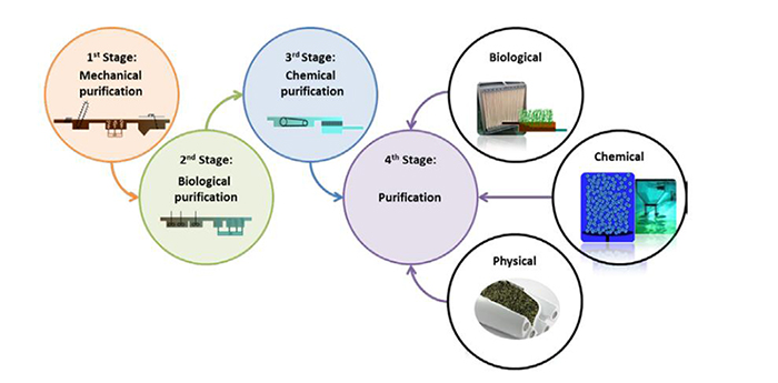
The ubiquitous presence of pharmaceuticals in the aquatic environment is a worldwide problem of today. Current analytical methods reveal ever more pharmaceuticals in different water bodies. The concentrations in waters that are detectable reach nano-and picogram ranges, i.e., ppb and ppt levels. Observed concentrations amount to as high as few micrograms. Among the major entry paths are wastewater treatment plants, which are often unable to eliminate the pharmaceuticals sufficiently relying on their three conventional purification stages. Hence, pharmaceuticals enter the aquatic environment without desirable deconstruction. Thus, advanced wastewater treatment processes are under development to retain or eliminate these trace contaminants. According to Decision 2018/840, a watchlist of 15 contaminants of significant interest has been established for the monitoring of surface waters in the European Union. The contaminants include biocides and pharmaceuticals, among them three estrogens, estrone (E1), 17-β-estradiol (E2) and 17-α-ethinylestradiol, (EE2), the antibiotics azithromycin, clarithromycin and erythromycin of macrolide type, ciprofloxacin and amoxicillin of fluoroquinolone and betalactame type. This review will provide an overview of the currently explored and researched methods for the realization of a fourth purification stage in wastewater treatment plants. To this purpose, biological, chemical and physical purification processes are reviewed and their characteristics and potential discussed. The degradation efficacy of the pharmaceuticals on the EU-Watch list will be compared and evaluated with respect to the most promising processes, which might be realized on large scale. Last but not least, recent and novel pilot plants will be presented and discussed.
Citation: Melanie Voigt, Alexander Wirtz, Kerstin Hoffmann-Jacobsen, Martin Jaeger. Prior art for the development of a fourth purification stage in wastewater treatment plant for the elimination of anthropogenic micropollutants-a short-review[J]. AIMS Environmental Science, 2020, 7(1): 69-98. doi: 10.3934/environsci.2020005
The ubiquitous presence of pharmaceuticals in the aquatic environment is a worldwide problem of today. Current analytical methods reveal ever more pharmaceuticals in different water bodies. The concentrations in waters that are detectable reach nano-and picogram ranges, i.e., ppb and ppt levels. Observed concentrations amount to as high as few micrograms. Among the major entry paths are wastewater treatment plants, which are often unable to eliminate the pharmaceuticals sufficiently relying on their three conventional purification stages. Hence, pharmaceuticals enter the aquatic environment without desirable deconstruction. Thus, advanced wastewater treatment processes are under development to retain or eliminate these trace contaminants. According to Decision 2018/840, a watchlist of 15 contaminants of significant interest has been established for the monitoring of surface waters in the European Union. The contaminants include biocides and pharmaceuticals, among them three estrogens, estrone (E1), 17-β-estradiol (E2) and 17-α-ethinylestradiol, (EE2), the antibiotics azithromycin, clarithromycin and erythromycin of macrolide type, ciprofloxacin and amoxicillin of fluoroquinolone and betalactame type. This review will provide an overview of the currently explored and researched methods for the realization of a fourth purification stage in wastewater treatment plants. To this purpose, biological, chemical and physical purification processes are reviewed and their characteristics and potential discussed. The degradation efficacy of the pharmaceuticals on the EU-Watch list will be compared and evaluated with respect to the most promising processes, which might be realized on large scale. Last but not least, recent and novel pilot plants will be presented and discussed.

| [1] | Tijani JO, Fatoba OO, Petrik LF (2013) A review of pharmaceuticals and endocrine-disrupting compounds: Sources, effects, removal, and detections. Water Air Soil Pollut 224. |
| [2] |
Gerbersdorf SU, Cimatoribus C, Class H, et al. (2015) Anthropogenic Trace Compounds (ATCs) in aquatic habitats-Research needs on sources, fate, detection and toxicity to ensure timely elimination strategies and risk management. Environ Int 79: 85-105. doi: 10.1016/j.envint.2015.03.011

|
| [3] |
Burke V, Richter D, Greskowiak J, et al. (2016) Occurrence of Antibiotics in Surface and Groundwater of a Drinking Water Catchment Area in Germany. Water Environ Res 88: 652-659. doi: 10.2175/106143016X14609975746604
|
| [4] |
Schwarzenbach RP (2006) The Challenge of Micropollutants in Aquatic Systems. Science 313: 1072-1077. doi: 10.1126/science.1127291
|
| [5] |
Luo Y, Guo W, Ngo HH, et al. (2014) A review on the occurrence of micropollutants in the aquatic environment and their fate and removal during wastewater treatment. Sci Total Environ 473-474: 619-641. doi: 10.1016/j.scitotenv.2013.12.065
|
| [6] |
Haddad T, Baginska E, Kümmerer K (2015) Transformation products of antibiotic and cytostatic drugs in the aquatic cycle that result from effluent treatment and abiotic/biotic reactions in the environment: An increasing challenge calling for higher emphasis on measures at the beginning of the pi. Water Res 72: 75-126. doi: 10.1016/j.watres.2014.12.042
|
| [7] |
Rivera-Utrilla J, Sánchez-Polo M, Ferro-García MÁ, et al. (2013) Pharmaceuticals as emerging contaminants and their removal from water. A review. Chemosphere 93: 1268-1287. doi: 10.1016/j.chemosphere.2013.07.059
|
| [8] |
Kümmerer K (2009) Antibiotics in the aquatic environment-a review-part I. Chemosphere 75: 417-434. doi: 10.1016/j.chemosphere.2008.11.086
|
| [9] |
Novo A, Andre S, Viana P, et al. (2013) Antibiotic resistance, antimicrobial residues and bacterial community composition in urban wastewater. Water Res 47: 1875-1887. doi: 10.1016/j.watres.2013.01.010
|
| [10] |
Margot J, Rossi L, Barry DA, et al. (2015) A review of the fate of micropollutants in wastewater treatment plants. Wiley Interdiscip Rev Water 2: 457-487. doi: 10.1002/wat2.1090
|
| [11] |
Sui Q, Cao X, Lu S, et al. (2015) Occurrence, sources and fate of pharmaceuticals and personal care products in the groundwater: A review. Emerg Contam 1: 14-24. doi: 10.1016/j.emcon.2015.07.001
|
| [12] |
Du B, Price AE, Scott WC, et al. (2014) Science of the Total Environment Comparison of contaminants of emerging concern removal, discharge, and water quality hazards among centralized and on-site wastewater treatment system ef fl uents receiving common wastewater in fl uent. Sci Total Environ 466-467: 976-984. doi: 10.1016/j.scitotenv.2013.07.126
|
| [13] | Decision 2018/840 (2018) Commission Implementing Decision (EU) 2018/840 of 5 June 2018 establishing a watch list of substances for Union-wide monitoring in the field of water policy pursuant to Directive 2008/105/EC of the European Parliament and of the Council and repealing Comm. |
| [14] | Directive 2000/60/EC (2000) Directive 2000/60/EC of the European Parliament and of the Council of 23 October 2000 establishing a framework for Community action in the field of water policy. |
| [15] | Directive 2008/105/EC Environmental quality standards applicable to surface water. |
| [16] | Directive 2013/39/EU Directive 2013/39/EU of the European Parliament and of the Council of 12 August 2013 amending Directives 2000/60/EC and 2008/105/EC as regards priority substances in the field of water policy Text with EEA relevance. |
| [17] | Decision 2015/495/EU Commission Implementing Decision (EU) 2015/495 of 20 March 2015 establishing a watch list of substances for Union-wide monitoring in the field of water policy pursuant to Directive 2008/105/EC of the European Parliament and of the Council (notified under. |
| [18] | aus der Beek T, Weber FA, Bergmann A, et al. (2016) Pharmaceuticals in the environment: Global occurrence and potential cooperative action under the Strategic Approach to International Chemicals Management (SAICM). UBA Texte 67/2016. |
| [19] |
Gogoi A, Mazumder P, Kumar V, et al. (2018) Groundwater for Sustainable Development Occurrence and fate of emerging contaminants in water environment : A review. Groundw Sustain Dev 6: 169-180. doi: 10.1016/j.gsd.2017.12.009
|
| [20] |
Liu J, Dan X, Lu G, et al. (2018) Investigation of pharmaceutically active compounds in an urban receiving water: Occurrence, fate and environmental risk assessment. Ecotoxicol Environ Saf 154: 214-220. doi: 10.1016/j.ecoenv.2018.02.052
|
| [21] |
Zhang R, Zhang R, Yu K, et al. (2018) Occurrence, sources and transport of antibiotics in the surface water of coral reef regions in the South China Sea: Potential risk to coral growth. Environ Pollut 232: 450-457. doi: 10.1016/j.envpol.2017.09.064
|
| [22] |
Jelic A, Gros M, Ginebreda A, et al. (2011) Occurrence, partition and removal of pharmaceuticals in sewage water and sludge during wastewater treatment. Water Res 45: 1165-1176. doi: 10.1016/j.watres.2010.11.010
|
| [23] |
Biel-Maeso M, Baena-Nogueras RM, Corada-Fernández C, et al. (2018) Occurrence, distribution and environmental risk of pharmaceutically active compounds (PhACs) in coastal and ocean waters from the Gulf of Cadiz (SW Spain). Sci Total Environ 612: 649-659. doi: 10.1016/j.scitotenv.2017.08.279
|
| [24] |
Mirzaei R, Yunesian M, Nasseri S, et al. (2018) Occurrence and fate of most prescribed antibiotics in different water environments of Tehran, Iran. Sci Total Environ 619-620: 446-459. doi: 10.1016/j.scitotenv.2017.07.272
|
| [25] | Paredes L, Omil F, Lema JM, et al. (2018) What happens with organic micropollutants during UV disinfection in WWTPs? A global perspective from laboratory to full-scale. J Hazard Mater 342: 670-678. |
| [26] |
Kostich MS, Batt AL, Lazorchak JM (2014) Concentrations of prioritized pharmaceuticals in effluents from 50 large wastewater treatment plants in the US and implications for risk estimation. Environ Pollut 184: 354-359. doi: 10.1016/j.envpol.2013.09.013
|
| [27] |
Orias F, Perrodin Y (2013) Characterisation of the ecotoxicity of hospital effluents: A review. Sci Total Environ 454-455: 250-276. doi: 10.1016/j.scitotenv.2013.02.064
|
| [28] |
Botero-Coy AM, Martínez-Pachón D, Boix C, et al. (2018) 'An investigation into the occurrence and removal of pharmaceuticals in Colombian wastewater'. Sci Total Environ 642: 842-853. doi: 10.1016/j.scitotenv.2018.06.088
|
| [29] | Wang B, Dai G, Deng S, et al. (2017) Large-scale enzymatic membrane reactors for tetracycline degradation in WWTP effluents. Water Res 45: 1-11. |
| [30] |
Tiedeken EJ, Tahar A, McHugh B, et al. (2017) Monitoring, sources, receptors, and control measures for three European Union watch list substances of emerging concern in receiving waters-A 20 year systematic review. Sci Total Environ 574: 1140-1163. doi: 10.1016/j.scitotenv.2016.09.084
|
| [31] |
Oulton RL, Kohn T, Cwiertny DM (2010) Pharmaceuticals and personal care products in effluent matrices: A survey of transformation and removal during wastewater treatment and implications for wastewater management. J Environ Monit 12: 1956. doi: 10.1039/c0em00068j
|
| [32] | Ahmed MB, Zhou JL, Ngo HH, et al. (2016) Progress in the biological and chemical treatment technologies for emerging contaminant removal from wastewater: A critical review. J Hazard Mater 323: 274-298. |
| [33] |
Cecconet D, Molognoni D, Callegari A, et al. (2017) Biological combination processes for efficient removal of pharmaceutically active compounds from wastewater: A review and future perspectives. J Environ Chem Eng 5: 3590-3603. doi: 10.1016/j.jece.2017.07.020
|
| [34] | Bayona JM (2013) Removal of Pharmaceutical Compounds from Wastewater and Surface Water by Natural Treatments. 62. |
| [35] |
Cole S (1998) The Emergence of Treatment Wetlands. Environ Sci Technol 32: 218A-223A. doi: 10.1021/es9834733
|
| [36] |
Verlicchi P, Zambello E (2014) How efficient are constructed wetlands in removing pharmaceuticals from untreated and treated urban wastewaters? A review. Sci Total Environ 470-471: 1281-1306. doi: 10.1016/j.scitotenv.2013.10.085
|
| [37] |
Fountoulakis MS, Terzakis S, Chatzinotas A, et al. (2009) Pilot-scale comparison of constructed wetlands operated under high hydraulic loading rates and attached biofilm reactors for domestic wastewater treatment. Sci Total Environ 407: 2996-3003. doi: 10.1016/j.scitotenv.2009.01.005
|
| [38] |
Hijosa-Valsero M, Fink G, Schlüsener MP, et al. (2011) Removal of antibiotics from urban wastewater by constructed wetland optimization. Chemosphere 83: 713-719. doi: 10.1016/j.chemosphere.2011.02.004
|
| [39] |
Hijosa-Valsero M, Matamoros V, Martín-Villacorta J, et al. (2010) Assessment of full-scale natural systems for the removal of PPCPs from wastewater in small communities. Water Res 44: 1429-1439. doi: 10.1016/j.watres.2009.10.032
|
| [40] | Dai Y, Dan A, Yang Y, et al. (2016) Factors Affecting Behavior of Phenolic Endocrine Disruptors, Estrone and Estradiol, in Constructed Wetlands for Domestic Sewage Treatment. EnvironSciTechnol 50: 11844-11852. |
| [41] |
Song H, Nakano K, Taniguchi T, et al. (2009) Estrogen removal from treated municipal effluent in small-scale constructed wetland with different depth. Bioresour Technol 100: 2945-2951. doi: 10.1016/j.biortech.2009.01.045
|
| [42] |
Verlicchi P, Galletti A, Petrovic M, et al. (2013) Removal of selected pharmaceuticals from domestic wastewater in an activated sludge system followed by a horizontal subsurface flow bed-Analysis of their respective contributions. Sci Total Environ 454-455: 411-425. doi: 10.1016/j.scitotenv.2013.03.044
|
| [43] |
Song H-L, Yang X-L, Nakano K, et al. (2011) Elimination of estrogens and estrogenic activity from sewage treatment works effluents in subsurface and surface flow constructed wetlands. Int J Environ Anal Chem 91: 600-614. doi: 10.1080/03067319.2010.496046
|
| [44] |
Hu X, Bao Y, Hu J, et al. (2017) Occurrence of 25 pharmaceuticals in Taihu Lake and their removal from two urban drinking water treatment plants and a constructed wetland. Env Sci Pollut Res 24: 14889-14902. doi: 10.1007/s11356-017-8830-y
|
| [45] |
Kimura K, Hara H, Watanabe Y (2007) Elimination of selected acidic pharmaceuticals from municipal wastewater by an activated sludge system and membrane bioreactors. Environ Sci Technol 41: 3708-3714. doi: 10.1021/es061684z
|
| [46] |
Fazal S, Zhang B, Zhong Z, et al. (2015) Industrial Wastewater Treatment by Using MBR (Membrane Bioreactor) Review Study. J Environ Prot (Irvine, Calif) 06: 584-598. doi: 10.4236/jep.2015.66053
|
| [47] |
Carmosini N, Lee LS (2009) Ciprofloxacin sorption by dissolved organic carbon from reference and bio-waste materials. Chemosphere 77: 813-820. doi: 10.1016/j.chemosphere.2009.08.003
|
| [48] |
Zuehlke S, Duennbier U, Lesjean B, et al. (2006) Long-Term Comparison of Trace Organics Removal Performances Between Conventional and Membrane Activated Sludge Processes. Water Environ Res 78: 2480-2486. doi: 10.2175/106143006X111826
|
| [49] | Baumgarten S (2007) Membranbioreaktoren zur industriellen Abwasserreinigung. |
| [50] |
Janssens R, Mandal MK, Dubey KK, et al. (2017) Slurry photocatalytic membrane reactor technology for removal of pharmaceutical compounds from wastewater: Towards cytostatic drug elimination. Sci Total Environ 599-600: 612-626. doi: 10.1016/j.scitotenv.2017.03.253
|
| [51] |
Abass OK, Wu X, Guo Y, et al. (2015) Membrane Bioreactor in China: A Critical Review. Int J Membr Sci Technol 2: 29-47. doi: 10.15379/2410-1869.2015.02.02.04
|
| [52] |
Besha AT, Gebreyohannes AY, Tufa RA, et al. (2017) Removal of emerging micropollutants by activated sludge process and membrane bioreactors and the effects of micropollutants on membrane fouling: A review. J Environ Chem Eng 5: 2395-2414. doi: 10.1016/j.jece.2017.04.027
|
| [53] |
Fan H, Li J, Zhang L, et al. (2014) Contribution of sludge adsorption and biodegradation to the removal of five pharmaceuticals in a submerged membrane bioreactor. Biochem Eng J 88: 101-107. doi: 10.1016/j.bej.2014.04.008
|
| [54] |
Kovalova L, Siegrist H, Singer H, et al. (2012) Hospital wastewater treatment by membrane bioreactor: Performance and efficiency for organic micropollutant elimination. Environ Sci Technol 46: 1536-1545. doi: 10.1021/es203495d
|
| [55] | Le T, Ng C, Tran NH, et al. (2018) Removal of antibiotic residues, antibiotic resistant bacteria and antibiotic resistance genes in municipal wastewater by membrane bioreactor systems. Water Res 498-508. |
| [56] |
Zhang W, Ding L, Luo J, et al. (2016) Membrane fouling in photocatalytic membrane reactors (PMRs) for water and wastewater treatment: A critical review. Chem Eng J 302: 446-458. doi: 10.1016/j.cej.2016.05.071
|
| [57] |
Huang BC, Guan YF, Chen W, et al. (2017) Membrane fouling characteristics and mitigation in a coagulation-assisted microfiltration process for municipal wastewater pretreatment. Water Res 123: 216-223. doi: 10.1016/j.watres.2017.06.080
|
| [58] |
Liébana R, Arregui L, Belda I, et al. (2015) Membrane bioreactor wastewater treatment plants reveal diverse yeast and protist communities of potential significance in biofouling. Biofouling 31: 71-82. doi: 10.1080/08927014.2014.998206
|
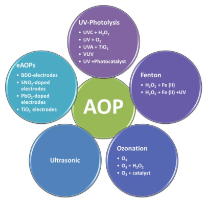
| [59] | Oppenländer T (2003) Photochemical Purification of Water and Air: Advanced Oxidation Processes (AOPs): Principles, Reaction Mechanisms, Reactor Concepts (Chemistry), Weinheim, WILEY-VCH Verlag. |
| [60] | Parsons S (2004) Advanced Oxidation Processes for Water and Wastewater Treatment, London, IWA Publishing. |
| [61] |
Andreozzi R, Caprio V, Insola A, et al. (1999) Advanced oxidation processes (AOP) for water purification and recovery. Catal Today 53: 51-59. doi: 10.1016/S0920-5861(99)00102-9
|
| [62] |
Voigt M, Bartels I, Nickisch-hartfiel A, et al. (2018) Elimination of macrolides in water bodies using photochemical oxidation. AIMS Environ Sci 5: 372-388. doi: 10.3934/environsci.2018.5.372
|
| [63] |
Homem V, Santos L (2011) Degradation and removal methods of antibiotics from aqueous matrices--a review. J Environ Manage 92: 2304-2347. doi: 10.1016/j.jenvman.2011.05.023
|
| [64] |
Monteagudo JM, Durán A, San Martín I (2014) Mineralization of wastewater from the pharmaceutical industry containing chloride ions by UV photolysis of H2O2/Fe(II) and ultrasonic irradiation. J Environ Manage 141: 61-69. doi: 10.1016/j.jenvman.2014.03.020
|
| [65] |
Shahidi D, Roy R, Azzouz A (2015) Advances in catalytic oxidation of organic pollutants-Prospects for thorough mineralization by natural clay catalysts. Appl Catal B Environ 174-175: 277-292. doi: 10.1016/j.apcatb.2015.02.042
|
| [66] | Brillas E (2014) A review on the degradation of organic pollutants in waters by UV photoelectro-fenton and solar photoelectro-fenton. J Braz Chem Soc 25: 393-417. |
| [67] |
Voigt M, Bartels I, Nickisch-Hartfiel A, et al. (2017) Photoinduced degradation of sulfonamides, kinetic, and structural characterization of transformation products and assessment of environmental toxicity. Toxicol Environ Chem 99: 1304-1327. doi: 10.1080/02772248.2017.1373777
|
| [68] |
Jelic a., Michael I, Achilleos a., et al. (2013) Transformation products and reaction pathways of carbamazepine during photocatalytic and sonophotocatalytic treatment. J Hazard Mater 263: 177-186. doi: 10.1016/j.jhazmat.2013.07.068
|
| [69] |
Vasconcelos TG, Henriques DM, König A, et al. (2009) Photo-degradation of the antimicrobial ciprofloxacin at high pH: Identification and biodegradability assessment of the primary by-products. Chemosphere 76: 487-493. doi: 10.1016/j.chemosphere.2009.03.022
|
| [70] | Suslick S, Fang M (1999) Acoustic cavitation and its chemical consequences. Phil Trans R Soc Lond A 335-353. |
| [71] | Torres-Palma RA, Serna-Galvis EA (2018) Sonolysis, Advanced Oxidation Processes for Waste Water Treatment, Elsevier, 177-213. |
| [72] |
Serna-Galvis EA, Botero-Coy AM, Martínez-Pachón D, et al. (2019) Degradation of seventeen contaminants of emerging concern in municipal wastewater effluents by sonochemical advanced oxidation processes. Water Res 154: 349-360. doi: 10.1016/j.watres.2019.01.045
|
| [73] |
Zoschke K, Börnick H, Worch E (2014) Vacuum-UV radiation at 185 nm in water treatment-a review. Water Res 52: 131-145. doi: 10.1016/j.watres.2013.12.034
|
| [74] |
Crapulli F, Santoro D, Sasges MR, et al. (2014) Mechanistic modeling of vacuum UV advanced oxidation process in an annular photoreactor. Water Res 64: 209-225. doi: 10.1016/j.watres.2014.06.048
|
| [75] | Heit G, Neuner A, Saugy P, et al. (1998) Vacuum-UV (172 nm) Actinometry. The Quantum Yield of the Photolysis of Water. J Phys Chem A 5639: 5551-5561. |
| [76] | Ratpukdi T (2014) Degradation of Paracetamol and Norfloxacin in Aqueous Solution Using Vacuum Ultraviolet (VUV) Process. J Clean Energy Technol 2: 168-170. |
| [77] |
Szabó RK, Megyeri C, Illés E, et al. (2011) Phototransformation of ibuprofen and ketoprofen in aqueous solutions. Chemosphere 84: 1658-1663. doi: 10.1016/j.chemosphere.2011.05.012
|
| [78] |
Voigt M, Jaeger M (2017) On the photodegradation of azithromycin, erythromycin and tylosin and their transformation products-A kinetic study. Sustain Chem Pharm 5: 131-140. doi: 10.1016/j.scp.2016.12.001
|
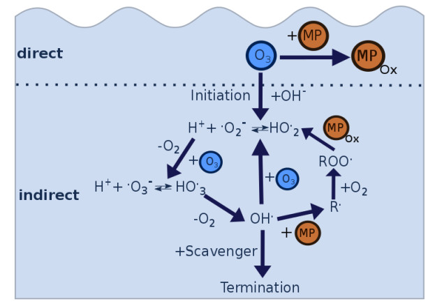
| [79] | Gottschalk C, Libra JA, Saupe A (2010) Ozonation of Water and Waste Water-A Practical Guide to Understanding Ozone and its Applications, Weinheim, WILEY-VCH Verlag GmbH & Co. KGaA. |
| [80] |
Antoniou MG, Hey G, Rodríguez Vega S, et al. (2013) Required ozone doses for removing pharmaceuticals from wastewater effluents. Sci Total Environ 456-457: 42-49. doi: 10.1016/j.scitotenv.2013.03.072
|
| [81] |
Ribeiro AR, Nunes OC, Pereira MFR, et al. (2015) An overview on the advanced oxidation processes applied for the treatment of water pollutants defined in the recently launched Directive 2013/39/EU. Environ Int 75: 33-51. doi: 10.1016/j.envint.2014.10.027
|
| [82] |
Matilainen A, Sillanpää M (2010) Removal of natural organic matter from drinking water by advanced oxidation processes. Chemosphere 80: 351-365. doi: 10.1016/j.chemosphere.2010.04.067
|
| [83] |
Tong L, Eichhorn P, Pérez S, et al. (2011) Photodegradation of azithromycin in various aqueous systems under simulated and natural solar radiation: kinetics and identification of photoproducts. Chemosphere 83: 340-348. doi: 10.1016/j.chemosphere.2010.12.025
|
| [84] |
Frontistis Z, Kouramanos M, Moraitis S, et al. (2015) UV and simulated solar photodegradation of 17α-ethynylestradiol in secondary-treated wastewater by hydrogen peroxide or iron addition. Catal Today 252: 84-92. doi: 10.1016/j.cattod.2014.10.012
|
| [85] |
Ma X, Zhang C, Deng J, et al. (2015) Simultaneous degradation of estrone, 17β-estradiol and 17α-ethinyl estradiol in an aqueous UV/H2o2 system. Int J Environ Res Public Health 12: 12016-12029. doi: 10.3390/ijerph121012016
|
| [86] |
Voigt M, Savelsberg C, Jaeger M (2017) Photodegradation of the antibiotic spiramycin studied by high-performance liquid quadrupole time-of-flight mass spectrometry. Toxicol Environ Chem 99: 624-640. doi: 10.1080/02772248.2017.1280039
|
| [87] | Hernández F, Bakker J, Bijlsma L, et al. (2019) The role of analytical chemistry in exposure science: Focus on the aquatic environment. Chemosphere 564-583. |
| [88] | Voigt M, Savelsberg C, Jaeger M (2018) Identification of Pharmaceuticals in The Aquatic Environment Using HPLC-ESI-Q-TOF-MS and Elimination of Erythromycin Through Photo-Induced Degradation. J Vis Exp. |
| [89] | Bobu M, Yediler A, Siminiceanu I, et al. (2013) Comparison of different advanced oxidation processes for the degradation of two fluoroquinolone antibiotics in aqueous solutions. J Environ Sci Heal Part A 48: 251-262. |
| [90] |
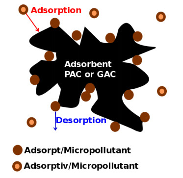
Yu F, Li Y, Han S, et al. (2016) Adsorptive removal of antibiotics from aqueous solution using carbon materials. Chemosphere 153: 365-385. doi: 10.1016/j.chemosphere.2016.03.083
|
| [91] |
Sharif F, Westerhoff P, Herckes P (2013) Sorption of trace organics and engineered nanomaterials onto wetland plant material. Environ Sci Process Impacts 15: 267-274. doi: 10.1039/C2EM30613A
|
| [92] |
Gao Y, Li Y, Zhang L, et al. (2012) Adsorption and removal of tetracycline antibiotics from aqueous solution by graphene oxide. J Colloid Interface Sci 368: 540-546. doi: 10.1016/j.jcis.2011.11.015
|
| [93] |
Mailler R, Gasperi J, Coquet Y, et al. (2016) Removal of emerging micropollutants from wastewater by activated carbon adsorption: Experimental study of different activated carbons and factors influencing the adsorption of micropollutants in wastewater. J Environ Chem Eng 4: 1102-1109. doi: 10.1016/j.jece.2016.01.018
|
| [94] | Kaub M, Biebersdorf N (2014) Kläranlage Höxter 4. Reinigungsstufe zur Elimination von Mikroschadstoffen, Bochum. |
| [95] |
Grover DP, Zhou JL, Frickers PE, et al. (2011) Improved removal of estrogenic and pharmaceutical compounds in sewage effluent by full scale granular activated carbon : Impact on receiving river water. J Hazard Mater 185: 1005-1011. doi: 10.1016/j.jhazmat.2010.10.005
|
| [96] |
Kovalova L, Siegrist H, Von Gunten U, et al. (2013) Elimination of micropollutants during post-treatment of hospital wastewater with powdered activated carbon, ozone, and UV. Environ Sci Technol 47: 7899-7908. doi: 10.1021/es400708w
|
| [97] |
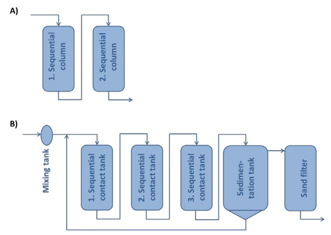
Mailler R, Gasperi J, Coquet Y, et al. (2016) Removal of a wide range of emerging pollutants from wastewater treatment plant discharges by micro-grain activated carbon in fluidized bed as tertiary treatment at large pilot scale. Sci Total Environ 542: 983-996. doi: 10.1016/j.scitotenv.2015.10.153
|
| [98] | Lima DRS, Baêta BEL, Aquino SF, et al. (2014) Removal of Pharmaceuticals and Endocrine Disruptor Compounds from Natural Waters by Clarification Associated with Powdered Activated Carbon. Water Air Soil Pollut 225. |
| [99] |
Rubirola A, Llorca M, Rodriguez-Mozaz S, et al. (2014) Characterization of metoprolol biodegradation and its transformation products generated in activated sludge batch experiments and in full scale WWTPs. Water Res 63: 21-32. doi: 10.1016/j.watres.2014.05.031
|
| [100] |
Kårelid V, Larsson G, Björlenius B (2017) Pilot-scale removal of pharmaceuticals in municipal wastewater: Comparison of granular and powdered activated carbon treatment at three wastewater treatment plants. J Environ Manage 193: 491-502. doi: 10.1016/j.jenvman.2017.02.042
|
| [101] |
Li L, Quinlivan PA, Knappe DRU (2002) Effects of activated carbon surface chemistry and pore structure on the adsorption of organic contaminants from aqueous solution. Carbon N Y 40: 2085-2100. doi: 10.1016/S0008-6223(02)00069-6
|
| [102] |
Benstoem F, Nahrstedt A, Boehler M, et al. (2017) Performance of granular activated carbon to remove micropollutants from municipal wastewater-A meta-analysis of pilot- and large-scale studies. Chemosphere 185: 105-118. doi: 10.1016/j.chemosphere.2017.06.118
|
| [103] | Margot J, Magnet A (2011) Elimination des micropolluants dans les eaux usées-Essais pilotes à la station d épuration de Lausanne. gwa 7: 487-493. |
| [104] |
Margot J, Kienle C, Magnet A, et al. (2013) Treatment of micropollutants in municipal wastewater: Ozone or powdered activated carbon? Sci Total Environ 461-462: 480-498. doi: 10.1016/j.scitotenv.2013.05.034
|
| [105] |
Baresel C, Malmborg J, Ek M, et al. (2016) Removal of pharmaceutical residues using ozonation as intermediate process step at Linköping WWTP, Sweden. Water Sci Technol 73: 2017-2024. doi: 10.2166/wst.2016.045
|
| [106] |
Mamo J, Insa S, Monclús H, et al. (2016) Fate of NDMA precursors through an MBR-NF pilot plant for urban wastewater reclamation and the effect of changing aeration conditions. Water Res 102: 383-393. doi: 10.1016/j.watres.2016.06.057
|
| [107] |
Hofman-Caris CHM, Siegers WG, van de Merlen K, et al. (2017) Removal of pharmaceuticals from WWTP effluent: Removal of EfOM followed by advanced oxidation. Chem Eng J 327: 514-521. doi: 10.1016/j.cej.2017.06.154
|
| [108] | Cédat B, de Brauer C, Métivier H, et al. (2016) Are UV photolysis and UV/H 2 O 2 process efficient to treat estrogens in waters? Chemical and biological assessment at pilot scale. Water Res 100: 357-366. |
| [109] |
El-taliawy H, Ekblad M, Nilsson F, et al. (2017) Ozonation efficiency in removing organic micro pollutants from wastewater with respect to hydraulic loading rates and different wastewaters. Chem Eng J 325: 310-321. doi: 10.1016/j.cej.2017.05.019
|
| [110] |
Ibáñez M, Borova V, Boix C, et al. (2017) UHPLC-QTOF MS screening of pharmaceuticals and their metabolites in treated wastewater samples from Athens. J Hazard Mater 323: 26-35. doi: 10.1016/j.jhazmat.2016.03.078
|
Figures(13) / Tables(8)

Melanie Voigt, Alexander Wirtz, Kerstin Hoffmann-Jacobsen, Martin Jaeger. Prior art for the development of a fourth purification stage in wastewater treatment plant for the elimination of anthropogenic micropollutants-a short-review[J]. AIMS Environmental Science, 2020, 7(1): 69-98. doi: 10.3934/environsci.2020005


 DownLoad: