The impact of hygienization as mild thermal pretreatment on the methane production of various organic wastes was investigated, including digestate issued from hydrolysis tank, thickened sludge from a municipal wastewater treatment plant (MWWTP sludge) and from a mixed domestic-industrial wastewater treatment plant (D-I WWTP sludge), sludge from a meat-processing plant (MP sludge), sieving rejection from a pork slaughterhouse, pork liver, cattle slurry, cattle scraping slurry and date seeds. They were thermally pretreated at 70 °C for one hour and subsequently put into AD digesters incubated at 37 °C for individual methane potential test. The modified Gompertz model was employed to evaluate the kinetic parameters of methane production curves (R2 = 0.944–0.999). The results were compared with the untreated samples. Significant enhancement of methane potentials induced by thermal treatment (p < 0.05) was observed when it comes to the pork liver (+8.6%), the slaughterhouse sieving rejection (+11.1%), the thickened MWWTP sludge (+12.5%) and the digestate issued from hydrolysis tank (+18.0%). The maximum methane production rates of the 4 substrates mentioned above were increased by thermal pretreatment as well (from 13.5% to 64%, p < 0.05). The lag time of the methane production was shortened for the digestate from hydrolysis tank and the MWWTP sludge (by 48.6% and 62.2% respectively, p < 0.05). No significant enhancement was obtained for the cattle slurry, the cattle scraping slurry and the D-I WWTP sludge. Additionally, the maximum methane production rate and the methane potential were reduced by thermal pretreatment for the MP sludge and the date seeds respectively (p < 0.05). In this paper, possible mechanisms were discussed to explain the different methane production behaviors of substrates after the mild thermal pretreatment.
1.
Introduction: Iterative continuous dynamical system
Some key processes in Nature can be viewed as iteratively continuous: within each iteration the process runs continuously reaching its final state that feeds into the next iteration. For example, in temperate areas, the growth of primary Producers is seasonal. During the growing season (usually Spring and Summer), plants continuously grow and compete. At the end of the season, some part of the plant biomass (e.g. leaves) falls and gets partially or fully decomposed, releasing nutrients into the soil. The released nutrients affect the plant growth and the competition outcomes in subsequent growing seasons. At larger scales, numerous phytoplankton species grow and compete in the upper ocean, the plankton biomass sinks to the deep ocean and decomposes, releasing nutrients into the water that the upwelling eventually brings to the upper ocean, thus affecting the growth and competition outcomes of new plankton.
Mathematically, such natural processes can be viewed as iterative dynamical systems, where the end state of each iteration affects the input parameters for the next iteration:
where:
F is the continuous function that governs the system dynamics within each iteration,
αi is the real-valued vector (or scalar) representing the input parameter(s), the values of which may vary between iterations (e.g. the supply of nutrients into the system);
X is the real-valued vector representing state variables (e.g. species density, nutrient stocks);
β is the real-valued vector (or scalar) representing biotic parameter(s) (e.g. species traits);
X0 represents the initial conditions of the state variables for each iteration (for simplicity, the initial conditions are assumed to be the same for all iterations but can be generalized to vary);
α0 represents the initial values of the input parameters for the first iteration;
Xi* is the end state of the i-th iteration, i.e. it is the solution X(T) at time T (the duration of each iteration) for dXdt=F(αi,β,X) with X(0) = X0; if T is sufficiently large and the solution approaches an equilibrium, then Xi* can be viewed as the equilibrium state of the i-th iteration;
g is the function that defines for each iteration (except the first one) the dependence of the input parameters on the end state of the previous iteration.
A more elaborate and interesting iterative system that captures not only nutrient feedbacks but also competitive and evolutionary outcomes can be introduced by allowing a biotic parameter (β, in this case a scalar) to vary, and then applying Adaptive Dynamics (Geritz et al., 1998 [7]; Diekmann, 2002 [5]) to track its evolution. Under certain conditions, Adaptive Dynamics allows using a single-species model to predict competitive outcomes of a multispecies system. For example, if system (1) has a positive globally stable equilibrium at each iteration, then the methods of Adaptive Dynamics can be applied to find the Evolutionary Steady (or Stable) Strategy (ESS) among all possible β values. This would be akin to considering a multispecies system with each species having a different trait β, and then finding among them the winner, if such exists. The winner's trait (or some function of it) can be taken as the end state of each iteration:
An alternative and more compact representation of (1a, b) is possible (without explicitly using function F, as a discrete dynamical system for αi), but the above structure has a couple of advantages. First, within each iteration it allows explicitly using a classical ecological model represented as dXdt=F(αi,βi,X). This makes the rich history of theoretical results for classical models applicable within iterations; it also allows experimenters to use conventional and well-tested set ups (e.g. chemostat) to track the dynamics within each iteration. Second, the most interesting part of the process, biologically, often rests in the continuous system dXdt=F(αi,βi,X) as illustrated with the case below.
2.
Iterative chemostat model
Let us start with a classical chemostat model (Smith and Waltman, 1995) [16] of the growth of one species on two limiting nutrients (substrates) in a well-mixed continuous culture, which will be later linked to the iterative system (1b):
Here:
N(t) and P(t) are the concentrations of nitrogen (N) and phosphorus (P), respectively, in the medium at time t;
X(t) is the biomass of the species at time t;
N0 and P0 are the inflowing concentrations of N and P, respectively;
d is the dilution (flow) rate (thus, 1d is the residence time of a molecule in the chemostat);
n and p are the N and P concentrations in the species biomass, respectively (also referred to, in the chemostat theory, as quotas or nutrient use efficiencies);
f(N,P) is the relative growth rate of the species.
The output of model (2) has no effect on its input. In ecological or physiological systems, however, the output of a process can and often does affect its input (feedback loops), e.g. through nutrient cycling or signaling. Extensions of the chemostat model accounting for some type of feedback (e.g. the experimenter manipulating the dilution rate depending on the internal state of the chemostat, the impulsive state feedback control, or linked chemostats) have been proposed and analyzed (e.g. Pirt and Kurowski, 1970 [13]; Codeço and Grover 2001 [2]; De Leenheer and Smith, 2003 [4]; Guo and Chen, 2009 [9]). Below, feedbacks between the supply of nutrients and the biotic parameters of the species are considered.
Apllying the notation used in (1b) to model (2), one can define X as (N, P, X) and F as the right-hand side of the classical chemostat model (2) with the input parameters being αi = (Ni0, Pi0) and the variable biotic parameter β being related to n/p, which is the ratio of nitrogen-to-phosphorus (N:P) of the species. Here is an example of the feedback loop: if system (2) represents the growth of a phytoplankton species in the upper ocean, then one can consider the set of all possible traits β, i.e. possible chemical compositions of a species that affect its N:P. Suppose that for a given supply of nutrients, the ESS value for β exists (under suitable conditions the ESS can be viewed as the trait of the species that outcompetes all others, i.e. the "winner"). Let us denote the ESS value of the winner as βi and take it as the end state of the i-th iteration. The biomass of the winner eventually sinks into the deep ocean, where it partially or fully decomposes, releasing N and P in the ratio that equals to, or strongly depends on, the N:P ratio of its biomass. The periodic upwelling brings those nutrients up from the deep ocean to the surface, thus, affecting the ratio of the nutrient supply, Ni+10:Pi+10, for the next growing season. In other words, at each iteration the ratio of input parameters, Ni+10:Pi+10, depends on the end state (βi) of the previous iteration: αi+1 = g(βi).
The above described iterative framework allows to raise questions that cannot be raised within the classical chemostat theory and it allows to do so in a mathematically rigorous way. For example, do sequences αi or βi exist and converge as i→∞? Such a question is not a mere mathematical curiosity but carries deep practical importance because it can potentially shed light on the evolution of nutrient ratios (stoichiometry) at the ecosystem or global scale, as outlined in the next section.
3.
The Redfield Ratio
The feedback between phytoplankton in the upper ocean and nutrients in the deep ocean is of special interest because it is responsible for what is likely to be the most expansive stoichiometric pattern on the planet, known as the Redfield ratio. The average N-to-P atomic ratio in phytoplankton in the upper ocean is ~16, i.e. for every atom of P there are about 16 atoms of N in the agammaegate phytoplankton biomass. Remarkably, nearly the same N:P ratio is found throughout the waters of the deep ocean in the both hemispheres. While considerable deviations from the Redfield ratio do exist, nevertheless, it shows surprising robustness on the vast spatial and temporal scales (Falkowski and Davis, 2004 [6]).
In the early 1930s, Alfred Redfield discovered the ratio after participating in the inaugural voyages of Atlantis—the first American ship built specifically for biological research. He first described the N:P ratio of 16 in Redfield (1934) [14] (later the ratio was extended to include carbon and other elements). However, it is still not fully understood why the N:P ratio centers around 16 and not some other biologically plausible number, and how this ratio can get established and persist on such large scales.
Several continuous dynamical models yielded insights into the Redfield ratio by considering feedbacks between the plankton dynamics and the nutrient pools. However, those models either explicitly introduce N:P = 16 into the model as an input parameter (e.g. Tyrrell 1999 [18]) or arrive at the conclusion that N:P = 16 has no inherent biological significance (e.g. Klausmeier et al., 2004 [11]). The latter seems to be at odds with Redfield's original hypothesis stating that the N:P = 16 is rooted in "protoplasm": "the relative proportion of phosphate and nitrate must tend to approach that characteristic of protoplasm in general and that, given time enough and freedom from systematic disturbing influences, a relationship between phosphate and nitrate such as that observed to occur in the sea must inevitably have arisen" (Redfield, 1934) [14]. To the best of my knowledge, no dynamic model exists that would explain the emergence and persistence of N:P ~16 without feeding into the model either N:P = 16 and/or several N:P value averaging to 16 (e.g. [18], Weber and Deutsch, 2012 [19]).
Here, an iterative-continuous chemostat model is developed that has a potential to show how N:P = 16 can emerge and persist from an arbitrary initial N:P condition in the ocean. In its present form, model (2) prescribes the N and P contents (quotas) to the phytoplankton, as biotic parameters n and p. This necessitates feeding into the model phenomenological N:P value (n:p) with no intrinsic biological significance. Below, I extend model (2), so that parameters n and p are not prescribed but, instead, arise from basic macromolecular values deeply shared by all life forms.
4.
Linking Chemostat Model to the Core Macromolecular Synthesis
For many microorganisms, and phytoplankton specifically, the largest or dominant pool of the intracellular N is protein, while the single largest pool of intracellular P often is ribosomal RNA (rRNA) (Sterner and Elser, 2002) [17]. These two genetic information-carrying biopolymers, protein and rRNA, are interdependent on their biosynthesis: rRNA (as a structural part of a ribosome) is required to synthesize proteins, while proteins (as RNA polymerases) are the ones that synthesize rRNAs. Below, I focus on these two biopolymers to understand their role in the Redfield ratio. The goal here is not to account for all the possible factors that can affect microbial N:P but rather understand if and how the interdependence of the two biopolymers leads to the rise and persistence of stoichiometric attractors, such as the Redfield ratio, on the ecosystem and evolutionary scales. While the proposed model ignores all other nutrient pools in the cell, it can be extended to include such pools but at the cost of increased complexity.
Here, I use the notation of Loladze and Elser (2011) [12] (also adopted by Daines et al., 2014 [3]), where the authors used the interdependence of protein and rRNA to derive the "Redfield formula" showing that the maximal possible microbial growth corresponds to N:P ~16, without feeding any specific N:P into the formula.
Let's characterize a microbial species by a trait defined here as the species protein:rRNA, β=a:r, where:
a and r are the species protein and rRNA contents, respectively.
The N and P contents in the species biomass can be directly expressed through its protein and rRNA contents via three stoichiometric constants universal to all life (na, nr, and pr):
where:
na = 0.17 and nr = 0.15 are the concentration of N in protein and rRNA, respectively, and pr = 0.09 is the concentration of P in rRNA.
A couple of notes. First, since protein has no P, it follows that the model assigns all the intracellular P to rRNA. Second, I do not and cannot use the term "constants" here with the same precision as physicists are so fortunate to be able to use for physical constants. Unlike, say, the speed of light in vacuum, the numerical value of "biological constants" (bioconstants), na, nr, and pr, can slightly vary depending on the relative frequency of amino acids in a protein or nucleotides in an rRNA. However, aside from such small variations, the three bioconstants are universally applicable to all biological matter, irrespective of its organizational complexity, be it a unicellular organism, a healthy or malignant tissue, or a population.
Next, the growth function, f(N,P), is linked to two fundamental macromolecular processes essential to any biological growth—protein and rRNA biogenesis. How does each of these two processes limit the overall growth?
If protein synthesis limits the overall growth, then the growth rate would be:
where γ is the variable rate of protein synthesis per unit mass of rRNA (all the protein in living systems is synthesized by ribosomes, each containing the fixed amount of rRNA; for details see Loladze and Elser (2011) [12]).
If rRNA synthesis limits the overall growth, then the growth rate would be:
where ψ is the variable rate of rRNA synthesis per unit mass of protein (all the RNA in living systems is synthesized by proteins, RNA polymerases).
The overall growth of the species then is limited by the lower of the two biosynthesis rates (5) and (6):
Next, the variable rates of protein and rRNA synthesis are linked to the availability of N and P in the medium. Many models of microbial growth focus on the uptake of nutrients and on the surface of the cell as the growth limiting step. While such surface-level limitations are important, the ultimate destination for the N and P atoms imported into a cell is protein and rRNA synthesis (the only pools considered here). A novel part of the model is that it shifts the focus for the growth limiting step from the uptake, which has been extensively studied and modeled in the literature, to the focal points of biogenesis related to genetic information—nucleic acids and protein. Recent empirical evidence shows that the supply of N and P affects key rates of biosynthesis in phytoplankton (Grosse et al., 2017 [8])—a feature that is underexplored in the plankton modeling literature but may be central for the Redfield ratio.
First, in the absence of N, no protein synthesis is possible, i.e. γ = 0. Second, under N-replete and otherwise optimal conditions, the synthesis of a protein is limited by the maximal capability of a ribosome to synthesize a protein. Let's denote the maximal possible protein synthesis rate per unit mass of rRNA as γm. It is reasonable to assume that the rate of protein synthesis increases with increasing N availability in the medium (N) from 0 (in the absence of N) to γm (N-replete conditions) in a smooth saturating fashion captured by Michaelis-Menten kinetics of nutrient uptake, also known as the Monod function for microbial growth:
where KN is the half-saturation constant defined as the N concentration in the medium corresponding to the protein synthesis rate being a half of γm.
A similar argument can be applied to the dependence of rRNA synthesis on P availability to arrive at:
where ψm is the maximal rate of rRNA synthesis per unit mass of protein, and KP is the half-saturation constant for P, defined as the P concentration in the medium corresponding to the rRNA synthesis rate being a half of ψm.
Substituting Eqs 8 and 9 into Eq 7 yields:
Note that in the absence of either nutrient, the species ceases to grow, irrespective of its β:
As shown in Loladze and Elser (2011) [12], the maximal rates of protein and rRNA synthesis, γm and ψm, can be deconstructed into eight molecular constants and rates, most of which are widely shared among organisms. The values for each of the eight parameters have been either theoretically derived or empirically determined (see Table 1), making no need to prescribe some arbitrary or theoretically convenient values to any of the eight parameters. Here is how γm and ψm are decomposed into the eight parameters:
where:
la is the number of amino acids in an RNA polymerase (Pol I holoenzyme for eukaryotes),
lr is the number of nucleotides in a ribosome,
ma is the average mass of an amino acid,
mr is the average mass of a ribonucleotide,
and the remaining four parameters are defined and determined at optimal and nutrient-replete conditions:
σa is the maximal peptide elongation rate (the number of amino acids added during synthesis to the growing protein chain per unit of time),
σr is the maximal rRNA elongation rate (the number of nucleotides added during synthesis to the growing rRNA per unit of time, and adjusted for excised external and internal transcribed spacers),
ϕa is the maximal fraction of ribosomes actively translating, i.e. synthesizing proteins,
ϕr is the maximal fraction of protein that is RNA polymerase actively transcribing DNA into rRNA, i.e. synthesizing rRNA.
Substituting Eqs 11 into Eq 10 yields the relative growth rate of the species as:
Substituting Eqs 3 and 4 into system (2) yields:
where f is defined by Eq 12.
System (12, 13) with 17 parameters has a remarkable property: 11 out the 17 parameters hold the same value (bioconstants) for either all (na, nr, pr) or several kingdoms of life (la, lr, ma, mr), or are widely applicable at least within each family or genus (σa, σr, ϕa, ϕr). Out of the remaining 6 parameters, KN and KP can be potentially species specific, and their variability is touched upon in Discussion. Parameter d (the dilution rate) reflects the physical properties of the system (the rate of inflow) rather than biological ones, leaving only three parameters (N0, P0, β) that would make biological sense to vary between iterations of the system.
This raises an interesting question directly related to the Redfield ratio: If the feedback between the nutrient supply N0 and P0, and the species protein:rRNA, β, is accounted for by the iterative framework, can the N:P ratio of either the supply or the species converge to some value? If so, is this value the Redfield ratio?
Rigorously formulating the above question requires to explicitly express the species N:P, denoted here as θ, through the species trait, protein:rRNA, β. This is straightforward to do using Eqs 3 and 4:
Eq 14 shows that θ is a one-to-one (linear) function of β and, hence, θ and β can be used interchangeably to refer to the species trait here (the reason for retaining both is to ease derivations).
Next, the iterative process is described. For each iteration, consider system (12, 13) in the positive cone (x, N, P) with all the 11 bioconstants set at their intrinsic values, and d set at some meaningful value. The remaining three parameters N0, P0, and β can vary as follows. For the first iteration (i = 1), the input parameters are set at some arbitrary ratio N10:P10. Among all the possible values of β, the ESS value is selected (assuming a unique ESS exists). It is possible to show that under reasonable conditions a unique ESS exists (I.L. and Sergei Pilyugin, unpublished data). Let us denote the ESS value for protein:rRNA as β1 for the first iteration. It uniquely defines the species N:P via Eq 14, denoted here as θ1, which is taken as the output of the first iteration.
For the second iteration (i = 2), the N:P ratio of the inflow, N20:P20 is set to θ1. This reflects the cycling of nutrients, where the biomass sinks and decomposes, releasing nutrients into the deep waters that the upwelling subsequently brings up to the upper ocean. With the nutrient supply for the second iteration being equal to θ1, system (12, 13) is again considered with all the possible β values, among which the ESS value is selected, denoted as β2. It defines the species N:P (θ2). For the next iteration (i = 3), the N:P of the inflow is set to θ2, and so on the iterations continue.
Questions then arise about the convergence of {θn}∞n=1. Does the sequence converge? If so, to what value? Is the value unique? Considering that most of the parameters in (12, 13) are immutable, what is the numerical value of the point of convergence, if such a point does exist? Is the value 16? If not, how far is the value from 16 and how does it depend on the core macromolecular parameters?
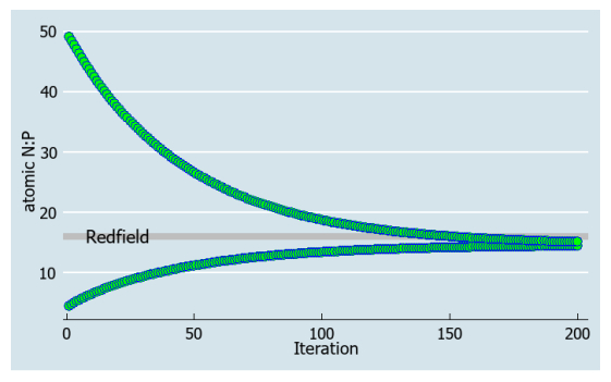
These questions can be schematically represented on Figure 1.
Summarizing the above, an iterative chemostat linked to the core biosynthesis can be formulated as follows:
and
N10:P10 is set at an arbitrary value, and:
where βi = ESS(β) for (15) at i-th iteration, if a unique ESS exists.
Table 1 lists values of the 11 bioconstants. Note that for any given i and β, system 15 is a classical chemostat model of one species growing on two limiting nutrients. Eq 16 describe the feedback: for the initial iteration, the inflow N:P ratio is set at some arbitrary value; for each subsequent iteration the ratio is equal to the N:P of the "winner" of the preceding iteration (θi) defined by its protein:rRNA (βi) via Eq 14.
The purpose of this paper is to introduce the interactive-continuous framework and, specifically, the iterative chemostat, which allows to mathematically formulate key questions related to the Redfield ratio. While answering these questions is outside of the scope of this paper, examples of numerical runs of system (15, 16) are given in Figure 2 depicting the N:P trajectories over many iterations. How the outcome of system (15, 16) depends on its variable parameters (d, KN, KP, Pi0) is touched upon in Discussion.
5.
Discussion
It is a canonic statement in ecology that energy flows but nutrients cycle. Yet, the richly developed set of ecological models, such as those in the population dynamics or the chemostat theory, often lack built-in feedbacks for nutrient cycling.
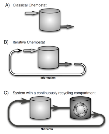
An iterative-continuous dynamical system introduced here can account for feedbacks found in ecological and physiological systems by making the input parameters at each iteration depend on the end state of the preceding iteration. While such dynamics can be mathematically formulated more concisely as a purely iterative system, the presented framework provides several advantages. First, the continuous function F in system (1a, b) retains the structure of classical ecological models that bring with them the rich theoretical and experimental history, thus, making well-established methods and results applicable within each iteration. Second, by accounting for feedbacks via iterations, the framework allows separating fast and slow time scales. For example, fast seasonal competitive dynamics in the upper ocean contrast with the slower nutrient cycling in the deep ocean, where nutrient residence time can be several hundred years. Alternative mathematical approaches exist for separating slow and fast time scales in ecological systems (e.g. Rinaldi and Scheffer, 2000 [15]; Klausmeier, 2010 [10]). The framework presented here specifically separates the slow feedback loop from the faster system dynamics. This makes it well-suited for experimental testing because it can eliminate the need for experimenters to explicitly set up the slow recycling compartment. Instead of physically feeding the nitrogen and phosphorus atoms from the output back to the input, the iterative chemostat (15, 16), passes only the information about their ratios, as shown in Figure 3. Experimenters can account for the feedback of the slow recycling compartment by periodically adjusting the N:P of the inflow based on the N:P of the outflow. This would allow them to track the slow evolution of nutrient ratios much faster than in natural systems.
However, the framework is not limited only to passing the information. System (1a, b) allows for broader range of feedbacks, including passing matter and for the recycling compartment itself to be continuous (via function g). The end state of each iteration can be taken as the value of the state variables (at an equilibrium or at some time T, the duration of each iteration) or as the value of biotic parameters corresponding to the ESS. The ESS value can be determined with the help of Adaptive Dynamics (Geritz et al., 1998 [7], Diekmann, 2004 [5]), allowing under suitable conditions to use a single-species system for modeling the outcome of multi-species competitive system.
The iterative chemostat (15, 16) allows to raise new questions that are difficult (or impossible) to raise rigorously within the classical non-iterative framework. As iterations progress, do stoichiometric ratios in the biomass or the medium converge to some value? If convergence to some point exists, it would mean that the point of convergence acts as a stoichiometric attractor to which the nutrient ratio in the ecosystem tend to over evolutionary scales. A particularly tantalizing possibility is that the stoichiometric N:P attractor is the famed Redfield ratio: more than 80 years after it was first described (Redfield, 1934)
[14], the ratio still leaves open key questions about the mechanisms responsible for both its emergence and its surprising robustness.
For the framework to be conducive for investigating the numerical value of the stoichiometric attractors (e.g. N:P = 16), the parameters in the continuous chemostat model are linked to key biopolymers and biosynthetic rates. The advantage of going to such a small organizational scale is twosome: 1) core macromolecular and biochemical processes are deeply shared among all life (e.g. transcription and translation), and 2) several "biological constants" exist at this scale that are otherwise extremely difficult to find at higher organization scales (e.g. most eukaryotes have the same number of ribonucleotides in a ribosome, but, on the organismal or population scale, it is hard to name a constant that would be as widely applicable to an entire kingdom of life as say lr, ma or pr are).
This allows to raise not only qualitative but also quantitative questions about the evolution of stoichiometric ratios. If across iterations, the N:P ratio in the biomass or the medium converges to some value, is that value 16? If not, how far is it from 16? How does it depend on the core bioconstants? Grosse et al. (2017) [8] empirically showed that biosynthetic rates in phytoplankton depend on the supply of N and P, which is the central feature of model (15, 16).
A peculiar feature of the Redfield ratio is that, while it is omnipresent on vast marine scales, it rarely persists in smaller bodies of water such as lakes. Does the persistence of the Redfield ratio depend on the strength of internal nutrient feedbacks and residence time of nutrients? The iterative framework allows to investigate such questions by varying the strength of the feedback between iterations via the dilution rate and absolute nutrient concentrations (d and Pi0).
Next, I discuss some limitations of the model, which considers only two cellular pools: protein and rRNA. While these pools often are the dominant N and P pools in microorganisms, other cell surface and intracellular N and P pools (e.g. phospholipids, storage compartments) can substantially impact the overall species N:P (e.g. Daines et al., 2014 [3]) and possibly affect the quantitative outcomes of iterations or the rate of convergence. However, the qualitative outcomes, such as the existence of points of convergence, i.e. stoichiometric attractors, might be robust to additions of various cellular N and P pools.
Another considerable simplification in the model is that it does not explicitly consider multiple steps that the N and P atoms go through before they become a part of the two biopolymers (protein or RNA). These steps include passive and/or active transport through the cell membrane and incorporation into monomers (amino acids or nucleotides). Each of these steps, together with environmental factors and limitations imposed by other nutrients, can affect species N:P. For example, Chrzanowski and Grover (2008) empirically showed that cell size and temperature can affect microbial N:P under the same nutrient supply [1]. The model presented here does not aspire to comprehensively account for the factors affecting plankton N:P but rather it sets a framework for investigating the emergence of stoichiometric attractors and their dependence on the core macromolecular machinery. Furthermore, model (15, 16) does not necessarily ignore the multiple steps that the N and P atoms go through before ending in proteins or rRNA but rather packs them into Monod functions (Eqs 8, 9 and 11) (a possibly relevant mathematical fact here is that an arbitrary number of compositions of Monod functions is a Monod function; Bo Deng personal communication).
The model considers only P as a limiting factor for rRNA synthesis, even though RNA is N-rich (nearly as N-rich as protein is, nr = 0.15 cf. na = 0.17), and, hence, N can potentially limit RNA synthesis. However, the atomic N:P ratio in RNA is very low (<4) and, under most realistic scenarios with the N:P of the inflow > 4, the N limitation of RNA synthesis is unlikely. While it is rather straightforward to add the N limitation of rRNA synthesis to model (15, 16), the resulting complications have no meaningful effect on the dynamics of the model under realistic scenarios (I.L. unpublished data).
The numerical runs in Figure 2 show the existence of a unique stoichiometric attractor to which the N:P in the system converges from arbitrary initial conditions either below or above the convergence point. Since the values of 11 bioconstants in the model (15, 16) are either theoretically or empirically derived, it leaves the numerical value of the stoichiometric attractor to potentially depend only on the variable parameters: the dilution rate, absolute nutrient concentrations or the two half-saturation constants. Interestingly, the model shows that the dilution rate correlates with the rate of convergence but has little effect on the value of the attractor. Similarly, richer nutrient levels slow down the convergence but have no affect on the value of the attractor. In other words, the convergence is iteratively faster in oligotrophic systems (such as are the interior parts of the ocean). The value of the attractor however, depends on the ratio of the half-saturation constants, KN:KP. This is expected because the half-saturation constants reflect multiple limitations that N and P atoms go through, all the way from the medium to the biopolymers. This may be prematurely interpreted as meaning that the complexity of nutrient uptake kinetics is ultimately driving the optimality of plankton N:P, and that the Redfield ratio carries no inherent biological significance. However, the Redfield formula in Loladze and Elser (2011) [12], which assumes nutrient replete and otherwise optimal conditions, does not depend on either KN or KP, but only on the 11 bioconstants:
I hypothesize that if under reasonable conditions the ratio of half-saturation constants can vary and evolve, it would also converge to the same value as the N:P of the attractor, and ultimately both ratios, driven by the ultimate demands of the biosynthetic machinery supported by the nutrient feedback, will converge to the Redfield ratio. If so, this would indicate that Alfred Redfield's original 1934 hypothesis that one of the planet's most expansive stoichiometric patterns, the N:P = 16, rises from the life's smallest organizational scale (the "characteristic of protoplasm") is true.
Acknowledgments
The author thanks James Grover and an anonymous referee for constructive reviews, Sergei Pilyugin for discussions about the proof of convergence, and Hal Smith for comments. The author acknowledges no funding for this work.
Conflict of interest
The author declares there is no conflict of interest


 DownLoad: