


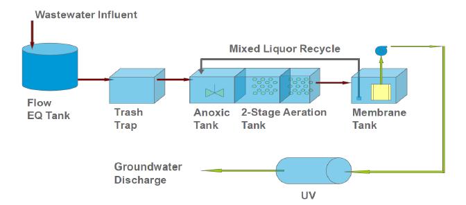
Figure 1.
System configuration.
Citation: Jianfeng Wen, Yanjin Liu, Yunjie Tu and Mark W. LeChevallier. Energy and chemical efficient nitrogen removal at a full-scale MBR water reuse facility[J]. AIMS Environmental Science, 2015, 2(1): 42-55. doi: 10.3934/environsci.2015.1.42
| [1] | Xinchang Guo, Jiahao Fan, Yan Liu . Maximum likelihood-based identification for FIR systems with binary observations and data tampering attacks. Electronic Research Archive, 2024, 32(6): 4181-4198. doi: 10.3934/era.2024188 |
| [2] | Shuang Yao, Dawei Zhang . A blockchain-based privacy-preserving transaction scheme with public verification and reliable audit. Electronic Research Archive, 2023, 31(2): 729-753. doi: 10.3934/era.2023036 |
| [3] | Yunfei Tan, Shuyu Li, Zehua Li . A privacy preserving recommendation and fraud detection method based on graph convolution. Electronic Research Archive, 2023, 31(12): 7559-7577. doi: 10.3934/era.2023382 |
| [4] | Qingjie Tan, Xujun Che, Shuhui Wu, Yaguan Qian, Yuanhong Tao . Privacy amplification for wireless federated learning with Rényi differential privacy and subsampling. Electronic Research Archive, 2023, 31(11): 7021-7039. doi: 10.3934/era.2023356 |
| [5] | Youqun Long, Jianhui Zhang, Gaoli Wang, Jie Fu . Hierarchical federated learning with global differential privacy. Electronic Research Archive, 2023, 31(7): 3741-3758. doi: 10.3934/era.2023190 |
| [6] | Wanshun Zhao, Kelin Li, Yanchao Shi . Exponential synchronization of neural networks with mixed delays under impulsive control. Electronic Research Archive, 2024, 32(9): 5287-5305. doi: 10.3934/era.2024244 |
| [7] | Yang Song, Beiyan Yang, Jimin Wang . Stability analysis and security control of nonlinear singular semi-Markov jump systems. Electronic Research Archive, 2025, 33(1): 1-25. doi: 10.3934/era.2025001 |
| [8] | Mohammed Alshehri . Blockchain-assisted cyber security in medical things using artificial intelligence. Electronic Research Archive, 2023, 31(2): 708-728. doi: 10.3934/era.2023035 |
| [9] | Mengjie Xu, Nuerken Saireke, Jimin Wang . Privacy-preserving distributed optimization algorithm for directed networks via state decomposition and external input. Electronic Research Archive, 2025, 33(3): 1429-1445. doi: 10.3934/era.2025067 |
| [10] | Seyha Ros, Prohim Tam, Inseok Song, Seungwoo Kang, Seokhoon Kim . A survey on state-of-the-art experimental simulations for privacy-preserving federated learning in intelligent networking. Electronic Research Archive, 2024, 32(2): 1333-1364. doi: 10.3934/era.2024062 |
In today's highly interconnected world, data privacy protection has become a critical concern across various application domains. Personal medical records, industrial control parameters, and even trade secrets are increasingly vulnerable to attacks or misuse [1,2,3,4]. When sensitive information is maliciously accessed or tampered with, it can lead not only to significant economic and societal losses but also to a destabilization of system security and stability. Therefore, the effective protection of data privacy and the prevention of unauthorized inferences and misuse of both individual and core information have become central issues of widespread interest in both academic and industrial circles [5,6,7].
The primary benefit of data privacy protection lies in its ability to intelligently mask, encrypt, or perturb personal and system-critical data, thereby preventing external attackers from reverse-engineering sensitive information. By implementing robust privacy-preserving techniques such as differential privacy, homomorphic encryption, and secure multi-party computation, organizations can effectively minimize security risks while maintaining the integrity and utility of the data. This ensures that individuals' personal privacy, corporate trade secrets, and other confidential information remain safeguarded during data collection, processing, analysis, and sharing. Moreover, a well-designed privacy protection framework fosters user trust, strengthens regulatory compliance, and enhances the overall resilience of digital systems against cyber threats, contributing to a more secure and sustainable data-driven ecosystem.
Over the years, researchers have developed various strategies for data security and privacy protection from both theoretical and practical perspectives. For instance, Rawat et al., in their exploration of cyber-physical systems (CPS) in smart grids and healthcare systems, emphasized the importance of security measures at both the network and physical layers for ensuring data confidentiality [8]. Ljung's systematic research on system identification laid the foundation for subsequent work on modeling and algorithmic optimization related to privacy protection and assessment [9]. Pouliquen et al. proposed a robust parameter estimation framework for scenarios with limited information based on binary measurements [10]. In a related study, Guo et al. developed an adaptive tracking approach for first-order systems using binary-valued observations with fixed thresholds, enhancing the accuracy of parameter estimation in constrained data environments [11]. The framework of local differential privacy had widely adopted in data statistics and analysis tasks, with comprehensive surveys that of Wang et al. demonstrating its crucial role in frequency estimation and machine learning applications under distributed settings [12]. Moreover, Ding et al. and Liu have each proposed methods for distributed control and networked predictive control in industrial CPS, embedding security and privacy requirements into real-time collaborative control processes [13,14]. In addition, Mahmoud et al. introduced a multi-layer defense approach for network attack modeling and vulnerability assessment, offering innovative solutions for maintaining data confidentiality against diverse threats [15]. Recent work by Taheri et al. explored differential privacy-driven adversarial attacks, like noise injection, to degrade deep learning-based malware detection, proposing defenses to enhance robustness [16]. In contrast, our differential privacy-based FIR system identification algorithm uses Laplace and randomized response mechanisms to encrypt data, ensuring parameter estimation accuracy in cyber-physical systems under privacy and security constraints.
In the realm of federated learning, data and model poisoning attacks pose significant challenges to the integrity and reliability of distributed systems, particularly impacting the accuracy of system identification processes. Nabavirazavi et al. proposed a randomization and mixture approach to enhance the robustness of federated learning against such attacks, demonstrating improved resilience in parameter estimation under adversarial conditions [17]. Similarly, Taheri et al. introduced robust aggregation functions to mitigate the effects of poisoned data, ensuring more reliable model updates in federated environments [18]. Nowroozi et al. exposed vulnerabilities in federated learning through data poisoning attacks, highlighting their detrimental impact on network security and the need for robust defenses to protect system dynamics [19]. Furthermore, Nabavirazavi et al. explored the impact of aggregation function randomization to counter model poisoning, emphasizing the importance of accurate parameter estimation despite malicious interventions [20]. These studies underscore the importance of accurate parameter estimation in adversarial environments. However, despite these advances in federated learning and privacy-preserving training, less attention has been paid to the fundamental task of system identification—an essential step for capturing system dynamics and ensuring the effectiveness of both attack detection and privacy protection strategies.
System identification is a key process in ensuring that attack detection and privacy protection measures are fully effective. Given the challenges of data tampering and privacy preservation, this paper focuses on the problem of data privacy protection from the perspective of system identification, specifically targeting the issue of data tampering under binary observation conditions [21,22].
System identification in the presence of binary observations and malicious tampering presents several challenges, including insufficient observational information, the presence of Gaussian noise combined with tampering interference, and the degradation of accuracy due to privacy noise [1,23]. First, binary observations significantly reduce the available data since they only give the relationship of size between the system output and a constant (called the threshold), increasing uncertainty in parameter estimation. The subtle changes in continuous signals may be ignored in binary observations, resulting in information loss and increasing the bias and variance of FIR system parameter estimation, thereby reducing system identification accuracy. Second, tampering by attackers can disrupt the data patterns critical for accurate identification. Finally, privacy encryption mechanisms, while protecting data sensitivity by introducing random noise, may negatively affect estimation accuracy. To address these challenges, this paper applies a dual encryption approach based on differential privacy to both the system input and binary output. This strategy not only prevents attackers from inferring or tampering with the data but also, through improved estimation algorithms and convergence analysis, achieves reliable system parameter identification, balancing the dual objectives of privacy protection and identification accuracy.
The paper proposes a dual differential privacy encryption strategy for system identification: First, Laplace noise is applied to the system input to prevent reverse-engineering of the system's structure or parameters. Then, binary observations are perturbed probabilistically to comply with differential privacy, protecting sensitive information at the output from being accessed or altered. An improved parameter estimation algorithm is introduced, with asymptotic analysis proving the strong consistency and convergence of the proposed method. Numerical simulations demonstrate that high identification accuracy can be maintained, even under various adversarial attack scenarios. This work offers a novel perspective and technical foundation for applying differential privacy in cyber-physical systems, addressing both data security and system identification needs.
This paper makes the following contributions:
● A differential privacy encryption algorithm for FIR system inputs is proposed, enhancing data privacy and security.
● A differential privacy encryption strategy under binary observation conditions is investigated, presenting a discrete 0-1 sequence differential privacy encryption method.
● Parameter estimation results under differential privacy encryption are validated, demonstrating the effectiveness of the proposed method in ensuring both data security and accurate system identification.
The rest of this paper is organized as follows: Section 2 introduces the FIR system model and discusses the data tampering threats under binary observations, formally stating the research problem. Section 3 details the dual differential privacy encryption methods for both input and output, along with the corresponding random noise models. Section 4 presents the parameter identification algorithm based on encrypted observation signals, accompanied by convergence analysis and strong consistency proofs. Section 5 explores the relationship between encryption budget and identification accuracy, presenting an optimization approach using Lagrange multipliers to determine the optimal encryption strength. Section 6 provides numerical simulations and compares results. Section 7 summarizes the work and discusses future research directions.
The object of this study is a single-input single-output finite impulse response (FIR) system, and its model is given below:
| $ yk=a1uk+a2uk−1+⋯+anuk−n+1+dk, $ | (1) |
which can be simplified to the following form:
| $ yk=ϕTkθ+dk,k=1,2,…, $ | (2) |
where $ u_k $ is the system input, $ \phi_k = [u_k, u_{k-1}, \dots, u_{k-n+1}]^T $ is the regression vector composed of the input signals, and $ \theta = [a_1, a_2, \dots, a_n]^T $ is the system parameter to be estimated for the system. $ d_k $ is independent and identically distributed Gaussian noise, with a mean of 0 and variance $ \sigma^2 $.
The output $ y_k $ is measured by a binary sensor with a threshold $ C $, and the resulting binary observation is
| $ s0k=I{yk≤C}={1,yk≤C,0,otherwise. $ | (3) |
The binary observation model $ s^0_k = I_{\{y_k \leq C\}} $ reflects a realistic scenario where only thresholded information is available from sensors. This situation arises frequently in practical FIR systems deployed in industrial monitoring or smart grid applications, where energy-efficient or low-cost sensors output only one-bit comparisons. The observation signal $ s_k^0 $ is transmitted through the network to the estimation center, but during the transmission process, it may be subject to data tampering by malicious attackers.
The signal $ s_k'' $ received by the estimation center is different from the original signal $ s_k^0 $, and the relationship between them is given by:
| $ Pr(s″k=0|s0k=1)=p,Pr(s″k=1|s0k=0)=q. $ | (4) |
We abbreviate the above data tampering attack strategy as $ (p, q) $. In this case, the estimation center estimates the system parameter $ \theta $ based on the received signal $ s_k'' $ [24,25].
Remark 2.1 Specifically, $ p $ denotes the probability that an original output of 0 is maliciously flipped to 1, and $ q $ denotes the probability that an original output of 1 is flipped to 0. These parameters characterize a probabilistic tampering model in which binary-valued observations are subject to asymmetric flipping attacks.
Remark 2.2 Binary quantization affects both noise characteristics and system identification accuracy: the additive noise becomes nonlinearly embedded in the binary output, and each observation carries limited information.
Differential privacy is a powerful privacy protection mechanism, and its core idea is to add random noise to the query results, limiting the impact of a single data point on the output, thus ensuring that attackers cannot infer individual information by observing the output. This process not only ensures that the system's input and output data are not directly accessed by attackers, but also effectively prevents attackers from reverse-engineering sensitive system information through input data.
The use of differential privacy in FIR also has its pros and cons. Using differential privacy-based encryption algorithms can limit the impact of data tampering attacks on the FIR system, but encryption itself involves adding noise, which can also lead to data tampering. Therefore, designing an encryption algorithm that meets both the accuracy requirements for parameter estimation and the need to limit data tampering attacks is the key focus of our research.
Figure 1 presents the end-to-end workflow of the proposed privacy-preserving FIR system identification framework under potential data tampering attacks. The process begins with the input signal $ u_k $, which is passed through a Laplace mechanism $ \operatorname{Lap}(\Delta u/\epsilon) $ to produce a perturbed input $ u_k' $, ensuring differential privacy at the input level. This perturbed input, together with the system's internal dynamics and additive noise $ d_k $, is processed by the FIR system to produce the output $ y_k $. The output is then passed through a binary-valued sensor that generates a thresholded observation $ s_k^0 = I\{y_k \leq C\} $. To preserve output-side privacy, $ s_k^0 $ is further randomized via a randomized response mechanism, resulting in $ s_k^{0'} $. This privatized observation is then transmitted over a communication network that may be subject to data tampering. During transmission, an attacker may flip the value of $ s_k^{0'} $ with certain probabilities, yielding the final corrupted observation $ s_k^{\prime\prime} $, which is received by the estimation center. The estimation center then applies a robust identification algorithm to estimate the unknown system parameters based on the received data. This pipeline integrates input perturbation, output privatization, and robustness against data manipulation into a unified privacy-preserving system identification framework.
This paper aims to address the following two questions:
● How can the harm caused by data tampering be mitigated or prevented through differential privacy algorithms?
● How can we design a parameter estimation algorithm, and what are the parameter estimation algorithm and the optimal differential privacy algorithm?
In this section, we consider an adversarial setting where the collected input-output data may be subject to tampering by untrusted components or compromised observers. Unlike traditional cryptographic methods such as MACs or digital signatures, which aim to detect and reject tampered data, our approach leverages differential privacy as a proactive defense. By adding calibrated randomness to both input and output channels, the encrypted signals inherently reduce the effectiveness of tampered data and enhance the robustness of system identification against malicious interference.
We first provide the standard definition of differential privacy. Let $ F $ be a randomized algorithm. For any two neighboring datasets $ x $ and $ x' $, their output results satisfy the following inequality:
| $ Pr(F(x)=S)Pr(F(x′)=S)≤eε. $ | (5) |
Here, $ S $ is a possible output of the algorithm, and $ \varepsilon $ is the privacy budget, which measures the degree of difference between the output distributions of the algorithm [1,23]. To ensure the privacy of the input data $ u_{i} $ in the FIR system, we encrypt the input signal using the Laplace mechanism of differential privacy. The Laplace mechanism was selected for input encryption due to its strong $ \varepsilon $-differential privacy guarantee, fitting the bounded input signals of FIR systems. The Gaussian mechanism, among others, offering weaker $ (\varepsilon, \delta) $-differential privacy or may not be suitable for FIR application, was considered unsuitable.
By adding Laplace noise to $ u_{i} $, we have:
| $ u′i=ui+Lap(Δuiε0), $ | (6) |
where $ Lap\left(\frac{\Delta u_i}{\epsilon_0}\right) $ denotes a random variable drawn from the Laplace distribution with mean 0 and scale parameter $ b = \frac{\Delta u_i}{\epsilon_0} $. The probability density function of the Laplace distribution is given by:
| $ Lap(x∣b)=12bexp(−|x|b),x∈R, $ | (7) |
where $ \Delta u_{i} $ is the sensitivity of the input $ u_{i} $, representing the maximum change in the system's input, and the privacy budget $ \varepsilon_0 $ determines the magnitude of the noise. The sensitivity $ \Delta f $ is used to measure the maximum change of the query function $ f $ over neighboring datasets, defined as
| $ Δf=maxx,x′‖f(x)−f(x′)‖, $ | (8) |
where $ x $ and $ x' $ are neighboring datasets differing by only one row. From Eq (8), we can derive that
| $ Δui=maxuk,u′k|yk−y′k|, $ | (9) |
where $ y_{k} $ and $ y_{k}' $ are the system outputs corresponding to the current input $ u_{k} $ and its neighboring input $ u'_{k} $, respectively, as described by Eq (1). Substituting this in, we can get
| $ Δui=maxuk,u′k|n−1∑i=0ai+1⋅(uk−i−u′k−i)|. $ | (10) |
If the distance between the neighboring input sets $ u_{k} $ and $ u'_{k} $ is a fixed value $ o $ (or $ o $ is the chosen mean), the sensitivity can be expressed as
| $ Δui=|n−1∑i=0ai+1⋅o|. $ | (11) |
Therefore, from Eqs (6) and (11), the encrypted result after adding noise to $ u_{i} $ is
| $ u′i=ui+Lap(|∑n−1i=0ai+1⋅o|ε0). $ | (12) |
After encrypting the input $ u_{i} $, the regression vector $ \phi_k = [u_k, u_{k-1}, \dots, u_{k-n+1}]^T $ formed by the input signals will also be affected by the Laplace noise. Let the noise vector be $ L_k = \left[l_1, l_2, \dots, l_n \right]^T $, where $ l_i = Lap\left(\frac{\Delta u_{i}}{\varepsilon_0} \right) $. The encrypted regression vector is
| $ ϕ′k=ϕk+Lk. $ | (13) |
Substituting the encrypted $ \phi_k' $ into the system output expression Eq (2), we obtain the encrypted system output
| $ y′k=(ϕk+Lk)Tθ+dk=ϕTkθ+LTkθ+dk. $ | (14) |
This implies that the statistical properties of the system output change under the influence of Laplace noise. By binarizing the system output $ y_k' $, we obtain the observed signal $ s_k^0 $. Assume we have a binary sensor with threshold $ C $, which converts $ y_k' $ into the binarized observation $ s_k^0 $ :
| $ s0k=I{y′k≤C}={1,y′k≤C,0,otherwise. $ | (15) |
Based on Eqs (14) and (13), the center will estimate the system parameter $ \theta $ based on the binarized signal $ s_k^0 $. By combining the tampered signal, the output $ s_k^0 $ can be expressed as
| $ s0k=I{ϕTkθ+LTkθ+dk≤C}. $ | (16) |
By introducing Laplace noise, we ensure the privacy of the system input $ u_i $. In the following sections, we will continue to discuss how to encrypt $ s_k^0 $ under the differential privacy mechanism and estimate the system parameter $ \theta $ under data tampering attacks.
In the system, we define $ \Pr(s_k^0 = 1) = \lambda_k $, which represents the probability that the signal $ s_k^0 $ equals 1 in each period $ n $. To protect this probability information, we apply differential privacy encryption to $ s_k^0 $. Specifically, for each $ s_k^0 $, there is a probability $ \gamma $ of retaining the original value, and with probability $ 1-\gamma $, we perform a negation operation. This operation can be formalized as
| $ s0′k={s0k,with probability γ,1−s0k,with probability 1−γ. $ | (17) |
This encryption process introduces randomness and achieves the goal of differential privacy. This encryption method effectively ensures that, whether $ s_k^0 $ is 0 or 1, an external attacker would find it difficult to infer the original value of $ s_k^0 $ by observing $ s_k^{0'} $, thus protecting data privacy. We have
| $ Pr(s0′k=1)=λk⋅γ+(1−λk)⋅(1−γ),Pr(s0′k=0)=(1−λk)⋅γ+λk⋅(1−γ). $ | (18) |
To analyze the encrypted $ s_k^0 $, we construct its likelihood function $ L $ to correct the perturbed encryption results. The likelihood function can be expressed as
| $ L=[λk⋅γ+(1−λk)(1−γ)]m⋅[(1−λk)⋅γ+λk(1−γ)]n−m, $ | (19) |
where $ m = \sum_{i = 1}^n X_i $ represents the observed number of times $ s_k^{0'} = 1 $, and $ X_i $ is the value of the $ i $ -th encrypted signal $ s_k^{0'} $. By maximizing this likelihood function, we can estimate the maximum likelihood estimate for $ \lambda_k $ after encryption. The maximization process leads to the estimation formula
| $ ^λk=γ−12γ−1+12γ−1⋅∑ni=1Xin. $ | (20) |
This estimate expresses the effect of the encrypted $ s_k^{0'} $ on the true $ \lambda_k $.
To further analyze the unbiasedness of the estimate, we can analyze the mathematical expectation and prove that the estimate is unbiased. The specific derivation is as follows:
| $ E(^λk)=12γ−1[γ−1+1nn∑i=1Xi]=λk. $ | (21) |
Based on the unbiased estimate, we can obtain the expected number $ N $ of signals equal to 1 in each period $ n $ as
| $ N=^λk×n=γ−12γ−1n+12γ−1⋅n∑i=1Xi. $ | (22) |
According to the definition of differential privacy, the relationship between the privacy parameter $ \varepsilon_0 $ and $ \gamma $ is
| $ γ≤eε1⋅(1−γ). $ | (23) |
By further derivation, we can obtain the calculation formula for the privacy budget $ \varepsilon_0 $ as
| $ ε1=ln(γ1−γ). $ | (24) |
Through the above encryption mechanism [12], we ensure that the system satisfies differential privacy while maintaining high robustness against interference from attackers on the observation of $ s_k $. During data transmission, the observed value $ s_k^0 $ may be subjected to attacks, and the tampering probability of the observed value $ s_k^0 $ is
| $ {Pr(s″k=0|s0′k=1)=p,Pr(s″k=1|s0′k=0)=q. $ | (25) |
Assume that the system input $ \{ u_k \} $ is periodic with a period of $ n $, i.e.,
| $ uk+n=uk. $ | (26) |
Let $ \pi_1 = \phi_1'^T, \pi_2 = \phi_2'^T, \dots, \pi_n = \phi_n'^T $, and the cyclic matrix formed by $ u_k $ is
| $ Φ=[πT1,πT2,⋯,πTn]T. $ | (27) |
After the preservation process applied to both inputs and outputs of $ u_k $ and $ s_k^0 $, during data transmission, the observed value $ s_k^0 $ will be attacked, and both active and passive attacks on the encrypted data will be limited and disturbed by noise. In the next section, we will provide a parameter estimation algorithm.
Under external attacks, and in the sense of the Cramér-Rao lower bound, the optimal estimation algorithm for the encrypted parameter $ \widehat{\theta}_N $ is given below:
| $ ˆθN=Φ−1[ξN,1,…,ξN,n]T, $ | (28) |
| $ ξN,i=C−F−1(1LNLN∑l=1s″(l−1)n+i), $ | (29) |
where $ \Phi^{-1} $ is the inverse matrix in Eq (27), $ C $ is the threshold in Eq (3), $ F^{-1} $ is the inverse cumulative distribution function, and $ s''_{(l-1)n+i} $ is the doubly encrypted $ s_k^0 $ in each period. For a data length $ N $, it is divided into $ L_N = \left\lfloor \frac{N}{n} \right\rfloor $, which is the integer part of $ N $ divided by the input period $ n $, representing the number of data segments $ L_N $ [26].
Definition 4.1 An algorithm is said to have strong consistency if the estimated value $ \hat{\theta}_N $ produced by the algorithm satisfies that as the sample size $ N \to \infty $, the estimate converges to the true value of the parameter $ \theta $ (or the encrypted true value $ \bar{\theta} $) with probability 1, i.e., $ \hat{\theta}_N \to \theta \text{ or } \hat{\theta}_N \to \bar{\theta} \, \text{w.p.1 as} \, N \to \infty $.
This conclusion follows the analysis in [24], which establishes strong consistency of estimators under binary-valued observation and bounded noise conditions.
Theorem 4.1 For the parameter estimation under the attack strategy $ (p, q) $ in Eq (28) with encrypted conditions, the expanded form of the true value $ \bar{\theta} $ is
| $ ˆθN→ˉθ=Φ−1[C−F−1((2γ−1)(1−p−q)FZ1(C−πT1θ)+(1−p)(1−γ)+qγ),…,C−F−1((2γ−1)(1−p−q)FZn(C−πTnθ)+(1−p)(1−γ)+qγ)]T $ | (30) |
and the algorithm has strong consistency. Here, $ \theta $ represents the parameter vector to be estimated in the system, and $ C $, $ \gamma $, $ \Phi^{-1} $, and $ \pi_k^T $ are given in Eqs (15), (17), and (27), respectively. $ F^{-1} $ is the inverse cumulative distribution function of noise $ d_k $, and $ F_{Z_k}(z) $ is the cumulative distribution function of the combined noise from Laplace noise $ l_k^T \cdot \theta $ and Gaussian noise $ d_k $.
Proof: Under data tampering attacks, in the period $ N $, each period's $ s_k'' $ is independent and identically distributed. For $ k = (l-1)n + i $, where $ i = 1, \ldots, n $, the regression vector $ \phi_k $ is periodic with period $ n $, i.e., $ \phi_{k+n} = \phi_k $. Define $ \pi_i = \phi_i $, so $ \phi_{(l-1)n + i} = \pi_i $. Since $ \phi_{(l-1)n + i} = \pi_i $, and the noise terms $ L_k $, $ d_k $ are i.i.d., the sequence $ \{ s_{(l-1)n + i}'' \}_{l = 1}^{L_N} $ is i.i.d. for each $ i $.
By the strong law of large numbers, for each $ i $ :
| $ 1LNLN∑l=1s″(l−1)n+i→E[s″(l−1)n+i]w.p.1 asN→∞. $ | (31) |
Next, we compute $ \mathbb{E}[s_{(l-1)n + i}''] $. Let $ k = (l-1)n + i $. The encrypted input is $ \phi_k' = \phi_k + L_k = \pi_i + L_k $, and the system output is:
| $ y′k=(πi+Lk)Tθ+dk=πTiθ+LTkθ+dk. $ | (32) |
Define $ Z_k = L_k^T \theta + d_k $. The binary signal is:
| $ s0k=I{y′k≤C}=I{πTiθ+Zk≤C}=I{Zk≤C−πTiθ}. $ | (33) |
Thus:
| $ λk=Pr(s0k=1)=Pr(Zk≤C−πTiθ)=FZi(C−πTiθ). $ | (34) |
The output encryption gives $ s_k^{0'} $ :
| $ E[s0′k]=γλk+(1−γ)(1−λk)=(2γ−1)λk+(1−γ). $ | (35) |
After the attack strategy $ (p, q) $ :
| $ E[s″k]=(1−p)E[s0′k]+q(1−E[s0′k])=(1−p−q)E[s0′k]+q. $ | (36) |
Substitute $ \mathbb{E}[s_k'] $ :
| $ E[s″k]=(1−p−q)[(2γ−1)FZi(C−πTiθ)+(1−γ)]+q. $ | (37) |
Simplify:
| $ E[s″k]=(2γ−1)(1−p−q)FZi(C−πTiθ)+(1−p)(1−γ)+qγ. $ | (38) |
Define:
| $ ηi=(2γ−1)(1−p−q)FZi(C−πTiθ)+(1−p)(1−γ)+qγ. $ | (39) |
Thus:
| $ 1LNLN∑l=1s″(l−1)n+i→ηiw.p.1. $ | (40) |
From the definition of $ \hat{\theta}_N $ :
| $ ξN,i=C−F−1(1LNLN∑l=1s″(l−1)n+i)→C−F−1(ηi)w.p.1. $ | (41) |
Therefore:
| $ ˉθN=Φ−1[ξN,1,…,ξN,n]T→Φ−1[C−F−1(η1),…,C−F−1(ηn)]T. $ | (42) |
Note that the total observation noise comprises the superposition of the original Gaussian noise $ d_k $ and the added Laplace noise due to differential privacy encryption. Since both noise sources are independent and have finite variance, their sum forms a new independent noise process with bounded second moments. This preserves the excitation condition needed for strong consistency. Here, the strong consistency follows from the strong law of large numbers. From Eqs (27)–(29) and (34), the expanded form of $ \bar{\theta} $ is obtained, thus completing the proof.
Our goal is to study how to maximize encryption within the permissible range of estimation errors.
To clarify the impact of different encryptions on the results, we analyze them separately based on the independence of input and output noise.
For the input noise encryption, the noise variance $ \sigma_L^2 $ introduced by input encryption, which affects $ \hat{\theta} $ through the system model, is as follows:
| $ D0=σ2L=2(1ε0)2n∑i=1(θiΔui)2. $ | (43) |
For the output noise encryption, since $ s'_k $ is a binary random variable, its variance is
| $ Var(s′k)=Pr(s′k=1)(1−Pr(s′k=1))=(1−γ+λk(2γ−1))(γ−λk(2γ−1)). $ | (44) |
From Eq (20), we can derive the variance of the maximum likelihood estimate $ \hat{\lambda}_k $ as
| $ Var(ˆλk)=(1(2γ−1)n)2n∑k=1Var(s′k). $ | (45) |
Substituting the result from Eq (44), we can get
| $ Var(ˆλk)=Var(s′k)(2γ−1)2n=(1−γ+λk(2γ−1))(γ−λk(2γ−1))(2γ−1)2n. $ | (46) |
The parameter estimate $ \hat{\theta} $ depends on $ \lambda_k $, and $ D_1 $ is defined as
| $ D1=Var(ˆλk)=(1−γ+λk(2γ−1))(γ−λk(2γ−1))(2γ−1)2n. $ | (47) |
To solve the optimal encryption problem, we model the optimization of the optimal encryption strategy:
| $ maxε0,ε1(D0+D1)s.t. ‖¯θ−θ‖≤ϵ, $ | (48) |
where $ \varepsilon_0 $ and $ \varepsilon_1 $ are the differential privacy budgets for input and output, respectively, and $ D_0 $ and $ D_1 $ are the functions that measure the impact of input and output encryption noise on the parameter estimate $ \bar{\theta} $, where $ D_0 = 2 \left(\frac{1}{\varepsilon_0} \right)^2 \sum_{i = 1}^n (\theta_i \Delta u_i)^2 $ and $ D_1 = \frac{\operatorname{Var}(s'_k)}{(2\gamma - 1)^2 n} $. $ \| \bar{\theta} - \theta \| $ is the parameter estimation error, which must be less than or equal to the given threshold $ \epsilon $, and both $ \bar{\theta} $ and $ \theta $ must be greater than zero.
Theorem 5.1 In the case of differential privacy with the preservation process applied to both inputs and outputs, $ \sigma_Z^2 $ is monotonically decreasing with respect to the privacy parameter of input $ \varepsilon_0 $, which indicates the smaller $ \varepsilon_0 $ is, the stronger the privacy protection provides, but the worse the estimation accuracy is.
Proof: $ L_k^T \theta $ is a linear combination of Laplace noise, and $ d_k $ is Gaussian noise, while $ Z_k $ is the sum of these two. Then, the variance of each $ l_i $ is
| $ Var(li)=2(Δuiε0)2. $ | (49) |
Thus,
| $ Var(LTkθ)=n∑i=1θ2iVar(li)=2(1ε0)2n∑i=1(θiΔui)2. $ | (50) |
The total variance of $ Z_k $ is
| $ σ2Z=Var(Zk)=Var(LTkθ)+Var(dk)=σ2L+σ2d, $ | (51) |
where
| $ σ2L=2(1ε0)2n∑i=1(θiΔui)2. $ | (52) |
To rigorously prove monotonicity, we can verify it by analyzing the derivative of $ \sigma_Z^2 $ with respect to $ \varepsilon_0 $. Taking the derivative of $ \sigma_Z^2 $ with respect to $ \varepsilon_0 $,
| $ dσ2Zdε0=ddε0(2(1ε0)2n∑i=1(θiΔui)2+σ2d). $ | (53) |
Since $ \sigma_d^2 $ is a constant and does not depend on $ \varepsilon_0 $, we get
| $ dσ2Zdε0=−41ε30n∑i=1(θiΔui)2. $ | (54) |
Since $ \varepsilon_0 > 0 $ and $ \sum_{i = 1}^n (\theta_i \Delta u_i)^2 > 0 $, we have $ \frac{d \sigma_Z^2}{d \varepsilon_0} < 0 $. This implies that as $ \varepsilon_0 $ increases, $ \sigma_Z^2 $ decreases monotonically. According to system estimation theory, as the noise variance decreases, the estimation accuracy improves. Therefore, as $ \varepsilon_0 $ increases, $ \sigma_Z^2 $ decreases, making the estimated result $ \hat{\theta} $ closer to the true value $ \theta $. This concludes the proof.
Theorem 5.2 In the case of differential privacy with the preservation process applied to both inputs and outputs, $ \bar{\theta} $ is monotonically decreasing with respect to $ \varepsilon_1 $. The smaller $ \varepsilon_1 $ is, the stronger the privacy protection provides.
Proof: From Eq (24), we have $ \gamma = \frac{e^{\varepsilon_1}}{e^{\varepsilon_1} + 1} $ and $ 2\gamma - 1 = \frac{e^{\varepsilon_1} - 1}{e^{\varepsilon_1} + 1} $.
Substituting into Eq (30), we can express $ \bar{\theta} $ as
| $ ˉθ=Φ−1[C−F−1(eε1−1eε1+1⋅FZ1(C−πT1θ)+1−FZ1(C−πT1θ)−eε1eε1+1),…,C−F−1(eε1−1eε1+1⋅FZn(C−πTnθ)+1−FZn(C−πTnθ)−eε1eε1+1)]T. $ | (55) |
By simplifying each term, we obtain
| $ (eε1−1)FZi(C−πTiθ)+(eε1+1)(1−FZi(C−πTiθ))−eε1eε1+1. $ | (56) |
Simplifying the numerator, it can be inferred that
| $ (eε1−1)FZi(C−πTiθ)+(eε1+1)(1−FZi(C−πTiθ))−eε1=eε1FZi(C−πTiθ)−FZi(C−πTiθ)+eε1+1−eε1FZi(C−πTiθ)−FZi(C−πTiθ)−eε1=−2FZi(C−πTiθ)+1. $ | (57) |
Substituting each term with $ \frac{-2 F_{Z_i}(C - \pi_i^T \theta) + 1}{e^{\varepsilon_1} + 1} $, the expression for $ \bar{\theta} $ becomes
| $ ˉθ=Φ−1[C−F−1(−2FZ1(C−πT1θ)+1eε1+1),…,C−F−1(−2FZn(C−πTnθ)+1eε1+1)]T. $ | (58) |
This concludes the proof.
In parameter estimation, the estimation error is typically related to the variance of the observation noise. Differential privacy encryption for both input and output introduces noise that affects the bias and variance of parameter estimation.
The expected value of the parameter estimate $ \hat{\theta} $ is $ \bar{\theta} $, i.e.,
| $ E[\hat{\theta}] = \bar{\theta}. $ |
The deviation between $ \bar{\theta} $ and the true parameter $ \theta $ is caused by the encryption noise. Our goal is to solve for $ \| \bar{\theta} - \theta \| $, and express it as a function of $ \varepsilon_0 $ and $ \varepsilon_1 $.
The mean square error (MSE) of the parameter estimate can be expressed as the square of the bias plus the variance:
| $ MSE(ˆθ)=‖E[ˆθ]−θ‖2+Var(ˆθ). $ | (59) |
Since we are concerned with the bias of the estimate $ \| \bar{\theta} - \theta \| $, and the variance of the estimate also depends on $ D_0 $ and $ D_1 $, we need to express both the bias and variance as functions of $ \varepsilon_0 $ and $ \varepsilon_1 $.
To accurately express $ \| \bar{\theta} - \theta \| $, we start from the root mean square error (RMSE):
| $ RMSE(ˆθ)=√trace(Var(ˆθ)). $ | (60) |
The total variance of the system's parameter estimate is
| $ Var(ˆθ)=(σ2d+D0+D1)(ΦTΦ)−1, $ | (61) |
where $ \sigma_d^2 $ is the system's inherent noise variance, $ D_0 $ and $ D_1 $ are the variances introduced by input and output encryption noise, and $ \Phi $ is the matrix from Eq (27).
Thus, the root mean square error of the estimate can be expressed as
| $ RMSE(ˆθ)=√trace((σ2d+D0+D1)(ΦTΦ)−1). $ | (62) |
Since $ \Phi^T \Phi $ is a known design matrix, we can represent the estimation error as
| $ ‖ˉθ−θ‖≤k√σ2d+D0+D1, $ | (63) |
where $ k = \sqrt{\operatorname{trace}((\Phi^T \Phi)^{-1})} $.
Based on the above derivation, the optimization problem can be reformulated as:
| $ maxε0,ε1D0+D1s.t.‖ˉθ−θ‖≤ϵσ2d+D0+D1≤ϵ2eff, $ |
where $ \epsilon_{\text{eff}}^2 = \epsilon^2 / k^2 - \sigma_d^2 $.
Now, we construct the Lagrangian objective function
| $ L(ε0,ε1,λ)=D0+D1−λ(D0+D1−ϵ2eff). $ | (64) |
For $ \varepsilon_0 $, we have
| $ D0=2(1ε0)2n∑i=1(θiΔui)2. $ | (65) |
Take partial derivatives with respect to $ \varepsilon_0 $, and we have
| $ ∂D0∂ε0=−4(1ε30)n∑i=1(θiΔui)2. $ | (66) |
For $ \varepsilon_1 $, we have
| $ D1=Var(s′k)(2γ−1)2n, $ | (67) |
where $ \gamma = \frac{e^{\varepsilon_1}}{e^{\varepsilon_1} + 1} $, and we can compute
| $ ∂γ∂ε1=eε1(eε1+1)2. $ | (68) |
Now, further differentiate $ D_1 $. First, rewrite $ D_1 $ as
| $ D1=Var(s0′k)(2γ−1)2n. $ | (69) |
Differentiate $ (2\gamma - 1)^2 $ with respect to $ \varepsilon_1 $, and it can be obtained that
| $ ∂∂ε1[(2γ−1)2]=4⋅(2γ−1)⋅eε1(eε1+1)2. $ | (70) |
Now, applying the chain rule, we have
| $ ∂D1∂ε1=−8Var(s0′k)⋅(2γ−1)eε1n(eε1+1)4. $ | (71) |
By the above analysis, the optimal values for $ \varepsilon_0 $ and $ \varepsilon_1 $ need to satisfy the following constraint:
| $ D0+D1=ϵ2eff. $ | (72) |
Taking partial derivatives with respect to $ \varepsilon_0 $ and $ \varepsilon_1 $, we get
| $ ∂L∂ε0=∂D0∂ε0−λ∂∂ε0(D0+D1)=0, $ | (73) |
| $ ∂L∂ε1=∂D1∂ε1−λ∂∂ε1(D0+D1)=0. $ | (74) |
Substituting the previously computed derivatives, we have
| $ −4(1ε30)n∑i=1(θiΔui)2−λ⋅0=0, $ | (75) |
| $ −8Var(s0′k)n⋅(2γ−1)eε1(eε1+1)4−λ⋅0=0. $ | (76) |
For $ \varepsilon_0 $, since $ \frac{\partial}{\partial \varepsilon_0}(D_0 + D_1) = 0 $, the derivative is completely determined by the objective function. To maximize the objective function under the constraint, we first check if the condition holds. Then, we can solve for $ \varepsilon_0 $ to satisfy the given constraint.
For $ \varepsilon_1 $, we also solve for $ \lambda $ to obtain the optimal solution.
The optimal solutions for $ \varepsilon_0 $ and $ \varepsilon_1 $ are
| $ ε0=√21+ϵ2eff, $ | (77) |
| $ ε1=23(1+ϵ2eff). $ | (78) |
Remark 5.1 These solutions are confirmed based on the value of $ \lambda $, and the specific numerical solution can be obtained through numerical computation.
Consider the following system:
| $ {yk=a1uk+a2uk−1+dk,sk=I{yk≤C},k=1,…,N, $ | (79) |
where $ a_1 = 10 $ and $ a_2 = 5 $ are the unknown parameters of the system, $ d_k $ is $ \mathcal{N}(0,100) $, and the threshold $ C = 7 $. The sample length for this simulation is set to $ N = 5000 $. The system input signals $ u_k $ are set as cyclic signals, with a value of $ [3, 5] $ in one cycle. The threshold $ \epsilon $ is set to 12. The sensitivity $ \Delta u $ is computed based on the maximum possible deviation between two neighboring input sequences, resulting in $ o = |5 - 3| = 2 $.
We encrypt the input signal $ u_k $ with Laplace noise under three different privacy budget parameters and simulate to verify its effects under different encryption strengths. According to the Laplace noise mechanism, the added noise follows the distribution:
| $ u′k=uk+Lap(Δuε), $ | (80) |
where $ u_k' $ is the encrypted input signal, $ \Delta u $ represents the sensitivity of the input signal, and $ \varepsilon $ is the privacy budget parameter.
Figure 2 shows the $ u_k $ signal under three different privacy budget parameters. The red line represents the strong encryption effect with a privacy budget of 0.1, the green line represents the moderate encryption effect with a privacy budget of 0.5, and the blue line represents the weak encryption effect with a privacy budget of 1.0. From the figure, it can be seen that as the privacy budget increases, the encryption strength decreases, and the amplitude of the noise significantly reduces. This result verifies the relationship between the strength of the Laplace noise and the privacy budget parameter.

From Figure 2, it can be observed that when the privacy budget parameter is small, i.e., under strong encryption, the noise amplitude is the largest, and the impact on the original signal $ u_k $ is most significant. On the other hand, under weak encryption, the noise amplitude is the smallest, and the impact on the original signal is minimal. The results of Laplace noise encryption at different strengths indicate that the stronger the encryption, the larger the noise amplitude, the more significant the interference on the original signal $ u_k $, and the better the privacy protection; the weaker the encryption, the smaller the noise amplitude, the less interference on the original signal, and the weaker the privacy protection.
The system output's binarized observation signal $ s_k $ has been encrypted with different privacy budget parameters. The encryption process introduces Laplace noise with varying strengths on the binarized $ s_k $ to protect privacy. After encryption, each $ s_k $ retains its original value with probability $ \gamma $ and is flipped with probability $ 1 - \gamma $. This process is expressed as
| $ s′k={sk,with probability γ,1−sk,with probability 1−γ. $ | (81) |
Figure 3 shows the binarized encrypted signal $ s_k' $ generated under three different privacy budget parameters ($ \varepsilon = 0.1 $, $ \varepsilon = 0.5 $, $ \varepsilon = 1.0 $), with the red, green, and blue lines corresponding to strong, moderate, and weak encryption effects, respectively.

From Figure 3, it is evident that the encryption strength significantly affects the degree of randomization of $ s_k' $. As the privacy budget parameter $ \varepsilon $ decreases (i.e., stronger encryption), the probability of flipping $ s_k' $ increases, leading to higher randomization of $ s_k' $. Conversely, when the privacy budget increases (i.e., weaker encryption), $ s_k' $ closely approximates the original binarized signal $ s_k $. This result verifies the relationship between encryption strength and signal randomization, namely, the stronger the encryption, the higher the randomization of $ s_k' $; the weaker the encryption, the more $ s_k' $ retains the pattern of the original signal.
Equation (30) provides the full expression for parameter estimation $ \widehat{\theta} $ under encryption, and we observe the accuracy of the parameter estimation in the simulation.
The selected privacy budget values are $ \varepsilon_0 = 1.0 $ and $ \varepsilon_1 = 1.0 $. The simulation results are shown in Figure 4, where, as the sample size increases, the parameter estimation approaches the encrypted value $ \bar{\theta} $.

We evaluate the impact of the privacy budget $ \varepsilon_0 $ encryption on the input $ u_k $ through simulations. Figure 5 shows the encryption effects under different privacy budgets. The error impact is represented by $ \left\| \widehat{\theta }-\theta \right\| $. The red line represents strong encryption with a privacy budget of 0.1, the green line represents moderate encryption with a privacy budget of 0.5, and the blue line represents weak encryption with a privacy budget of 1.0. From the error results, the simulation graph confirms the monotonicity Theorem 5.1. The smaller the privacy budget, the stronger the encryption, the larger the noise amplitude, and the greater the error between the estimated value and the true value. Conversely, when the privacy budget increases, the noise amplitude decreases, and the estimation error becomes smaller.

Next, we simulate the effect of adding differential privacy noise to the system output $ s_k $ and observe the impact of different privacy budget parameters $ \varepsilon_1 $ on the parameter estimation error. The simulation results are shown in Figure 6, which display the changes in parameter estimation error as the sample size varies for $ \varepsilon_1 = 0.1 $, $ \varepsilon_1 = 0.5 $, and $ \varepsilon_1 = 1.0 $. The result shown in Figure 6 is consistent with Theorem 5.2.

In this section, we further investigate how the magnitude of input signals affects the identification accuracy of FIR systems under dual differential privacy constraints. Specifically, both the input vector $ \boldsymbol{u}_k = [u_k, u_{k-1}]^\top $ and the binary-valued output $ s_k' $ are simultaneously perturbed by independent Laplace noise satisfying $ \epsilon $-differential privacy, denoted as $ \epsilon_0 $ and $ \epsilon_1 $, respectively.
To evaluate the estimation behavior under different input scales, we simulate two configurations: one using low-magnitude inputs $ (u_k, u_{k-1}) = (3, 5) $, and another using higher-magnitude inputs $ (30, 50) $, while keeping all other conditions identical (privacy budgets $ \epsilon_0 = \epsilon_1 = 0.5 $, threshold $ C = 70 $, and Gaussian noise variance $ \sigma^2 = 100 $).
The simulation results (Figure 7) reveal a significant contrast. While the lower magnitude input case results in relatively fluctuating estimation error due to stronger sensitivity to both noise and binarization, the higher input magnitude quickly leads to a nearly constant estimation error curve. This phenomenon is attributed to the high values of $ y_k = a_1 u_k + a_2 u_{k-1} + d_k $ being mostly above the threshold $ C $, rendering the binary outputs nearly constant and less informative for learning.

This experiment highlights the trade-off between input energy and privacy-resilient identifiability in FIR systems. It emphasizes the importance of designing input signals that balance observability with privacy-preserving distortion in binary measurement contexts.
We apply two noise distributions to the binarized output $ s_k' $ :
1) Gaussian noise: Zero mean, variance $ V = 1.0 $, standard deviation $ \sigma = \sqrt{V} = 1.0 $.
2) Laplacian noise: Zero mean, variance $ V = 1.0 $, scale parameter $ b = \sqrt{V / 2} \approx 0.707 $.
Both distributions maintain equal variance for a fair comparison. We simulate $ N = 5000 $ samples, adding Gaussian and Laplacian noise to $ s_k' $ and estimating parameters iteratively. The exponential moving average (EMA) of the estimation error is computed for both noise types.
Figure 8 presents the EMA estimation error for Gaussian and Laplacian noise over 5000 samples.

The results, shown in Figure 8, demonstrate that Laplacian noise yields higher estimation errors due to its heavier-tailed distribution, indicating stronger privacy protection at the cost of accuracy, thus validating the privacy-accuracy trade-off of our approach.
To investigate the impact of different privacy budget parameters $ \varepsilon_0 $ and $ \varepsilon_1 $ on the system parameter estimation, we adjust $ \varepsilon_0 $ and $ \varepsilon_1 $ to change the encryption strengths of the input and output, which affects both the estimation error and the degree of privacy protection in the system, thus helping to find the optimal solution.
Using the chain rule, we compute the partial derivatives of $ \varepsilon_0 $ and $ \varepsilon_1 $, i.e., $ \frac{\partial D_0}{\partial \varepsilon_0} = -\frac{2000}{\varepsilon_0^3} $ and $ \frac{\partial D_1}{\partial \varepsilon_1} = -\frac{8 \operatorname{Var}(s_k') (2\gamma - 1)e^{\varepsilon_1}}{n(e^{\varepsilon_1} + 1)^4} $. Through numerical methods, we solve for the optimal solution, and under the estimation error constraint $ \epsilon = 12 $, we calculate $ \epsilon_{\text{eff}}^2 = \frac{\epsilon^2}{k^2} - \sigma_d^2 $, yielding $ \epsilon_{\text{eff}}^2 \approx 4777 $. By setting the range for input encryption strength $ \varepsilon_0 $, combined with the optimization target and constraints, the optimal solution is found to be $ \varepsilon_0 \approx 4.3 $ and $ \varepsilon_1 \approx 0.07 $, with corresponding values of $ D_0 \approx 4598.9 $ and $ D_1 \approx 51.06 $.
We selected three different privacy budget parameter sets for comparison, as follows:
● Optimal solution: $ \varepsilon_0 = 4.3 $, $ \varepsilon_1 = 0.07 $.
● Scheme 1: $ \varepsilon_0 = 4.28 $, $ \varepsilon_1 = 0.2 $.
● Scheme 2: $ \varepsilon_0 = 5.0 $, $ \varepsilon_1 = 0.06 $.
For each parameter set, we calculated the corresponding $ D_0 $, $ D_1 $, and $ D_0 + D_1 $, and compared the parameter estimation errors.
The calculation results for the three parameter sets are summarized in the table below:
From Table 1, we can see that the optimal solution set yields the best overall encryption strength $ D_0 + D_1 $. This also corroborates that the optimal solution reaches the extremum, and to get even closer to the extremum, higher precision would be required. Moreover, this optimal solution does not focus on the trade-off between input and output, and if there are more specific requirements, additional constraints should be included in the solution process. If higher privacy protection strength is needed, the $ \epsilon $ limit can be relaxed to balance the encryption strengths for both input and output.
| Privacy budget parameters | $ D_0 $ | $ D_1 $ | $ D_0 + D_1 $ |
| Optimal solution ($ \varepsilon_0 = 4.3 $, $ \varepsilon_1 = 0.07 $) | 4598.9 | 51.06 | 4649.96 |
| Scheme 1 ($ \varepsilon_0 = 4.28 $, $ \varepsilon_1 = 0.2 $) | 4643.3 | 6.22 | 4649.52 |
| Scheme 2 ($ \varepsilon_0 = 5.0 $, $ \varepsilon_1 = 0.06 $) | 3400 | 69.47 | 3469.47 |
 DownLoad:
CSV
DownLoad:
CSV
This paper investigates the application of differential privacy encryption to reduce the risk of data tampering in FIR system identification under binary observation conditions. Two different differential privacy algorithms are proposed to ensure data security and privacy. The experimental evaluation confirms that the proposed method not only effectively protects sensitive information, but also maintains the accuracy of parameter estimation. These findings validate the effectiveness of the proposed scheme in this paper. Future work may explore optimizing the trade-off between privacy protection and estimation accuracy, as well as extending the approach to more complex system models and real-world applications.
The authors declare they have not used Artificial Intelligence (AI) tools in the creation of this article.
The authors declare no conflicts of interest in this paper.
| [1] |
Zhou H, Smith DW (2001) Advanced technologies in water and wastewater treatment. Can J Civil Eng 28: 49-66. doi: 10.1139/cjce-28-S1-49

|
| [2] |
Melin T, Jefferson B, Bixio D, et al. (2006) Membrane bioreactor technology for wastewater treatment and reuse. Desalination 187: 271-282. doi: 10.1016/j.desal.2005.04.086
|
| [3] | Verrecht B, Judd SJ, Guglielmi G, et al. (2008) An aeration energy model for an immersed membrane bioreactor. Water Res 42: 4716-4770. |
| [4] |
Schleper C, Nicol GW (2010) Ammonia-oxidising archaea - physiology, ecology and evolution. Adv Microb Physiol 57: 1-36. doi: 10.1016/B978-0-12-381045-8.00001-1
|
| [5] |
Giraldo E, Jjemba P, Liu Y, et al. (2011) Ammonia oxidizing archaea, AOA, population and kinetic changes in a full scale simultaneous nitrogen and phosphorus removal MBR. Proc Water Environ Federation 2011: 3156-3168. doi: 10.2175/193864711802721596
|
| [6] | Huang T, Li N, Huang Y (2012) Modelling of nitrogen removal and control strategy in continuous-flow-intermittent-aeration process. Afr J Biotechnol 11: 10626-10631. |
| [7] |
Guglielmi G, Andreottola G (2011) Alternate anoxic/aerobic operation for nitrogen removal in a membrane bioreactor for municipal wastewater treatment. Water Sci Techn 64: 1730-1735. doi: 10.2166/wst.2011.755
|
| [8] |
Curko J, Matosic M, Jakopovic HK, et al. (2010) Nitrogen removal in submerged MBR with intermittent aeration. Desalination Water Treat 24: 7-19. doi: 10.5004/dwt.2010.1118
|
| [9] |
Parikh C, Trivedi H, Livingston D (2011) A decade of simultaneous nitrification and denitrification experience in over 60 conventional and MBR applications - lessons learned. Proc Water Environ Federation 2011: 3629-3655. doi: 10.2175/193864711802721901
|
| [10] |
Holman JB, Wareham DG (2005) COD, ammonia and dissolved oxygen time profiles in the simultaneous nitrification/denitrification process. Biochem Eng J 22: 125-133. doi: 10.1016/j.bej.2004.09.001
|
| [11] |
Fu Z, Yang F, An Y, et al. (2009) Simultaneous nitrification and denitrification coupled with phosphorus removal in a modified anoxic/oxic-membrane bioreactor (A/O-MBR). Biochem Eng J 43: 191-196. doi: 10.1016/j.bej.2008.09.021
|
| [12] |
Li YZ, He YL, Ohandja DG, et al. (2008) Simutaneous nitrification-denitrification achieved by an improved internal-loop airlift MBR: comparative study. Bioresource Technol 99: 5867-5872. doi: 10.1016/j.biortech.2007.10.001
|
| [13] |
Sarioglu M, Insel G, Artan N, et al. (2009) Model evaluation of simultaneous nitrification and denitrification in a membrane bioreactor operated without an anoxic reactor. J Membrane Sci 337: 17-27. doi: 10.1016/j.memsci.2009.03.015
|
| [14] |
Wyffels S, Van Hulle SWH, Boeckx P, et al. (2004) Modelling and simulation of oxygen-limited partial nitrification in a membrane-assisted bioreactor (MBR). Biotechnol Bioeng 86: 531-542. doi: 10.1002/bit.20008
|
| [15] |
Daebel H, Manser R, Gujer W (2007) Exploring temporal variations of oxygen saturation constants of nitrifying bacteria. Water Res 41: 1094-1102. doi: 10.1016/j.watres.2006.11.011
|
| [16] |
Sharp R, Dailey S, Motyl M, et al. (2012) KDO experiments at NYC DEP's full-scale demonstration facility. Proc Water Environ Federation 2012: 4176-4182. doi: 10.2175/193864712811708482
|
| [17] |
Rieger L, Jones RM, Dold PL, et al. (2014) Ammonia-based feedforward and feeback aeration control in activated sludge process. Water Environ Res 86: 63-73. doi: 10.2175/106143013X13596524516987
|
| [18] | Henze M, Gujer W, Mino T, et al. (2000). Activated sludge models: ASM1, ASM2, ASM2d and ASM3. IWA Publishing, London. |
| [19] | Tchobanoglous G, Burton FL, Stensel HD (2004) Wastewater engineering, treatment and reuse, 4 Eds., Singapore: McGraw-Hill Education, 690. |
Figures(10) / Tables(1)

Jianfeng Wen, Yanjin Liu, Yunjie Tu and Mark W. LeChevallier. Energy and chemical efficient nitrogen removal at a full-scale MBR water reuse facility[J]. AIMS Environmental Science, 2015, 2(1): 42-55. doi: 10.3934/environsci.2015.1.42

| Privacy budget parameters | $ D_0 $ | $ D_1 $ | $ D_0 + D_1 $ |
| Optimal solution ($ \varepsilon_0 = 4.3 $, $ \varepsilon_1 = 0.07 $) | 4598.9 | 51.06 | 4649.96 |
| Scheme 1 ($ \varepsilon_0 = 4.28 $, $ \varepsilon_1 = 0.2 $) | 4643.3 | 6.22 | 4649.52 |
| Scheme 2 ($ \varepsilon_0 = 5.0 $, $ \varepsilon_1 = 0.06 $) | 3400 | 69.47 | 3469.47 |
DownLoad:
CSV
| Privacy budget parameters | $ D_0 $ | $ D_1 $ | $ D_0 + D_1 $ |
| Optimal solution ($ \varepsilon_0 = 4.3 $, $ \varepsilon_1 = 0.07 $) | 4598.9 | 51.06 | 4649.96 |
| Scheme 1 ($ \varepsilon_0 = 4.28 $, $ \varepsilon_1 = 0.2 $) | 4643.3 | 6.22 | 4649.52 |
| Scheme 2 ($ \varepsilon_0 = 5.0 $, $ \varepsilon_1 = 0.06 $) | 3400 | 69.47 | 3469.47 |
