Processing math: 100%
Research article Special Issues

A life cycle inventory analysis of wood pellets for greenhouse heating: a case study at Macdonald campus of McGill University1

  • Received: 10 July 2016 Accepted: 22 September 2016 Published: 29 September 2016
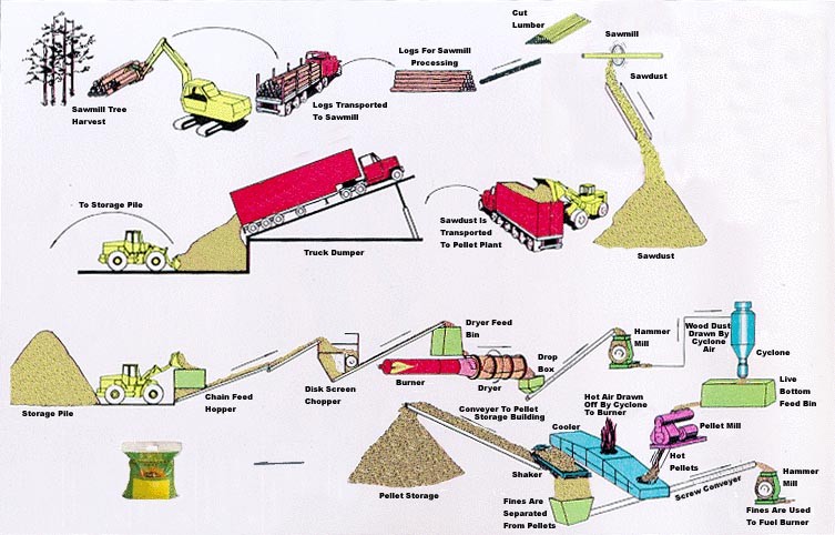
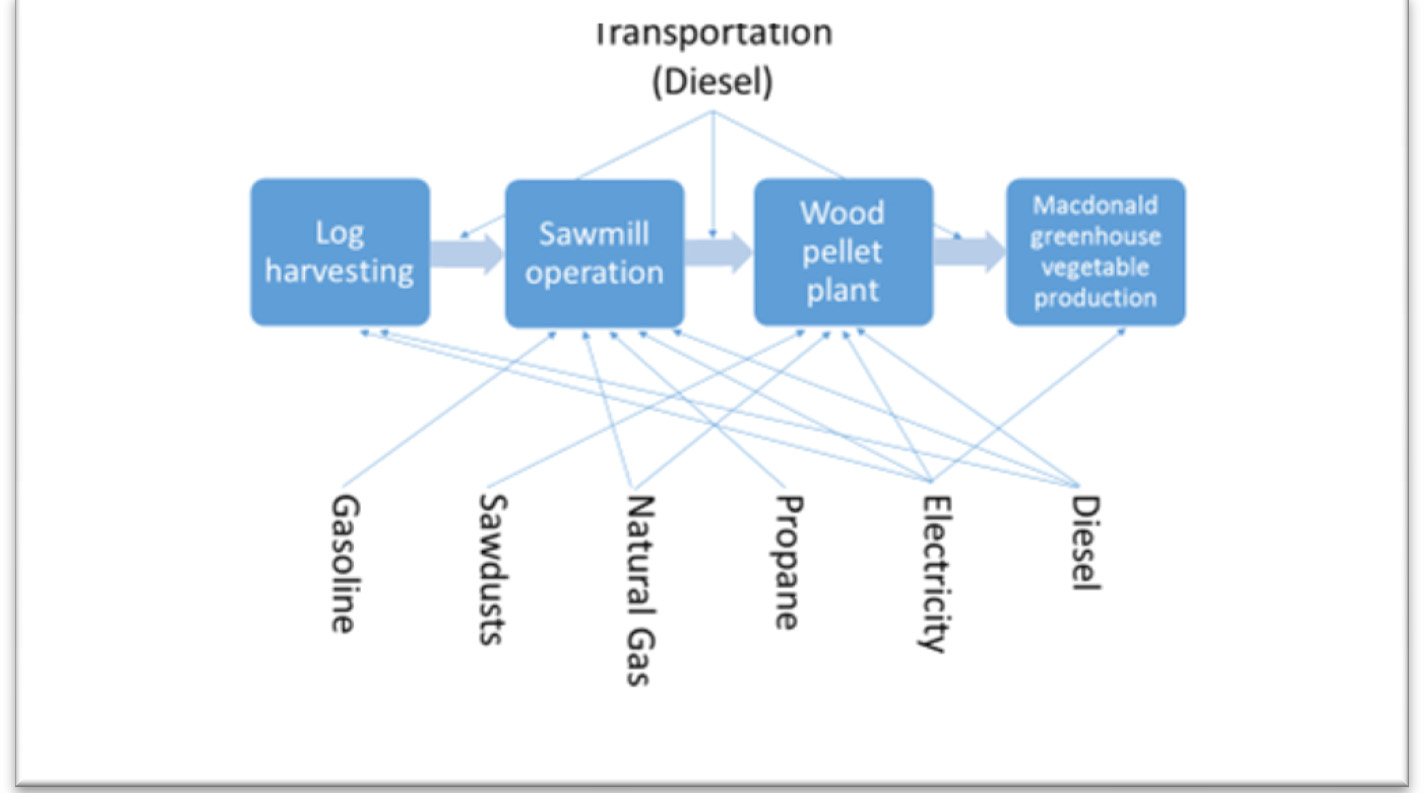
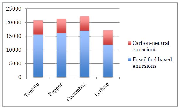
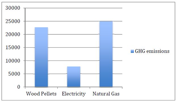
  • Wood pellets are one of the most promising alternatives to fossil fuel in Canada. Using wood pellets for heating allows saving on heating source expenses as compared to fossil fuels. Moreover, direct carbon emissions from wood pellets are regarded as carbon neutral since regrowth of vegetation captures and stores carbon that already exists in the atmosphere. Using wood pellets as a heating fuel for greenhouse vegetable production is expected to result in less greenhouse gas emissions than fossil fuels. Increasing the domestic consumption of wood pellets for greenhouse heating in Canada would reduce the environmental impact of energy consumption. This study investigates the potential of using wood pellets as an alternative fuel for commercial greenhouses in Quebec. This study applied a life-cycle analysis to demonstrate the energy flows and environmental consequences of using wood pellets for greenhouse vegetable production. The results found that greenhouse gas emissions from wood pellets are lower than natural gas in greenhouse operations.

    Citation: Tingting Wu, Kakali Mukhopadhyay, Paul J. Thomassin. A life cycle inventory analysis of wood pellets for greenhouse heating: a case study at Macdonald campus of McGill University1[J]. AIMS Energy, 2016, 4(5): 697-722. doi: 10.3934/energy.2016.5.697

    Related Papers:

    [1] Bo Sun, Ming Wei, Binbin Jing . Optimal model for the aircraft arrival and departure scheduling problem with fuzzy runway incursion time. Mathematical Biosciences and Engineering, 2021, 18(5): 6724-6738. doi: 10.3934/mbe.2021334
    [2] Ming Wei, Ligang Zhao, Zhijian Ye, Binbin Jing . An integrated optimization mode for multi-type aircraft flight scheduling and routing problem. Mathematical Biosciences and Engineering, 2020, 17(5): 4990-5004. doi: 10.3934/mbe.2020270
    [3] Bin Deng, Ran Ding, Jingfeng Li, Junfeng Huang, Kaiyi Tang, Weidong Li . Hybrid multi-objective metaheuristic algorithms for solving airline crew rostering problem with qualification and language. Mathematical Biosciences and Engineering, 2023, 20(1): 1460-1487. doi: 10.3934/mbe.2023066
    [4] Zilong Zhuang, Zhiyao Lu, Zizhao Huang, Chengliang Liu, Wei Qin . A novel complex network based dynamic rule selection approach for open shop scheduling problem with release dates. Mathematical Biosciences and Engineering, 2019, 16(5): 4491-4505. doi: 10.3934/mbe.2019224
    [5] Yafei Li, Yuxi Liu . Multi-airport system flight slot optimization method based on absolute fairness. Mathematical Biosciences and Engineering, 2023, 20(10): 17919-17948. doi: 10.3934/mbe.2023797
    [6] Bin Wang, Fagui Liu . Task arrival based energy efficient optimization in smart-IoT data center. Mathematical Biosciences and Engineering, 2021, 18(3): 2713-2732. doi: 10.3934/mbe.2021138
    [7] Shirin Ramezan Ghanbari, Behrouz Afshar-Nadjafi, Majid Sabzehparvar . Robust optimization of train scheduling with consideration of response actions to primary and secondary risks. Mathematical Biosciences and Engineering, 2023, 20(7): 13015-13035. doi: 10.3934/mbe.2023580
    [8] Santiago Iturriaga, Jonathan Muraña, Sergio Nesmachnow . Bio-inspired negotiation approach for smart-grid colocation datacenter operation. Mathematical Biosciences and Engineering, 2022, 19(3): 2403-2423. doi: 10.3934/mbe.2022111
    [9] Jianguo Duan, Mengting Wang, Qinglei Zhang, Jiyun Qin . Distributed shop scheduling: A comprehensive review on classifications, models and algorithms. Mathematical Biosciences and Engineering, 2023, 20(8): 15265-15308. doi: 10.3934/mbe.2023683
    [10] Yingjia Tan, Bo Sun, Li Guo, Binbin Jing . Novel model for integrated demand-responsive transit service considering rail transit schedule. Mathematical Biosciences and Engineering, 2022, 19(12): 12371-12386. doi: 10.3934/mbe.2022577
  • Wood pellets are one of the most promising alternatives to fossil fuel in Canada. Using wood pellets for heating allows saving on heating source expenses as compared to fossil fuels. Moreover, direct carbon emissions from wood pellets are regarded as carbon neutral since regrowth of vegetation captures and stores carbon that already exists in the atmosphere. Using wood pellets as a heating fuel for greenhouse vegetable production is expected to result in less greenhouse gas emissions than fossil fuels. Increasing the domestic consumption of wood pellets for greenhouse heating in Canada would reduce the environmental impact of energy consumption. This study investigates the potential of using wood pellets as an alternative fuel for commercial greenhouses in Quebec. This study applied a life-cycle analysis to demonstrate the energy flows and environmental consequences of using wood pellets for greenhouse vegetable production. The results found that greenhouse gas emissions from wood pellets are lower than natural gas in greenhouse operations.


    We consider the initial boundary value problem of the following porous elastic system with nonlinear or linear weak damping terms and nonlinear source terms

    {uttμuxxbϕx+g1(ut)=f1(u,ϕ),          x(0,L), t[0,T),ϕttδϕxx+bux+ξϕ+g2(ϕt)=f2(u,ϕ), x(0,L), t[0,T),u(x,0)=u0(x),  ut(x,0)=u1(x),             x(0,L),ϕ(x,0)=ϕ0(x),  ϕt(x,0)=ϕ1(x),            x(0,L),u(0,t)=u(L,t)=ϕ(0,t)=ϕ(L,t)=0,    t[0,T), (1.1)

    where u(x,t) and ϕ(x,t) are the displacement of the solid elastic material and the volume fraction, respectively, μ, b, δ and ξ are coefficients with physical meaning satisfying

    μ>0, b0, δ>0, ξ>0 and μξ>b2,

    u0, u1,ϕ0 and ϕ1 are given initial data, and the assumptions of weak damping terms g1, g2 and nonlinear source terms f1, f2 will be given in Section 2 by Assumption 2.1 and Assumption 2.2, respectively.

    In the physical view, elastic solid with voids is an important extension of the classical elasticity theory. It allows the processing of porous solids in which the matrix material is elastic and the interstices are void of material (see [8,20] and references therein). Porous media reflects the properties of many materials in the real world, including rocks, soil, wood, ceramics, pressed powder, bones, natural gas hydrates and so on. Due to the diversity of porous media and its special physical properties, such models were widely applied in the past few decades in the petroleum industry, engineering, etc (see [1,12,13,16,17,19]).

    As mathematical efforts, Goodman and Cowin [2,8] established the continuum theory and the variational principle of granular materials. Then Nunziato and Cowin [3,18] developed the linear and nonlinear theories of porous elastic materials. In recent years, the study of the porous elastic system also attracted a lot of attention [5,6,7,21,22]. We particularly mention that Freitas et.al. in [5] studied the problem (1.1) and proved the global existence and finite time blowup of solutions. Especially, they built up the continuous dependence on initial data of the local solution in the following version

    ˆE(t)eC0tˆE(0), C0>0, (1.2)

    which can also be extended to the global solution with the same form. By denoting z=(u,ϕ) and ˜z=(˜u,˜ϕ) the global solutions to problem (1.1) corresponding to the initial data z0, z1 and ˜z0, ˜z1, respectively, ˆE(0) is the distance of two sets of different initial data

    z0,˜z0V:=H10(0,L)×H10(0,L),

    and

    z1,˜z1L2(0,L)×L2(0,L),

    that is

    ˆE(0):=12z1˜z122+12z0˜z02V,

    and ˆE(t) is the distance of solutions induced by these two sets of different initial data

    ˆE(t):=12zt˜zt22+12z˜z2V.

    The growth estimate (1.2) indicates that the growth of the distance of solutions ˆE(t) is bounded by an exponential growth bound with time t. In other words, as the time t goes to infinity, the distance of solutions ˆE(t) of the system is bounded by a very large bound, by which it is hard to explain the solutions z and ˜z of such a dissipative system with the initial data z0,z1 and ˜z0,˜z1, respectively, as both of them are expected to decay to zero as the time t goes to infinity. Hence, the estimate on the growth of the distance of solutions ˆE(t) is proposed to be improved to reflect the decay properties with time t to be consistent with the dissipative behavior of the system. To achieve this, the efforts in the present paper are illustrated by two new continuous dependence results on the initial data for the global-in-time solution. Especially, it is found that the system with the linear damping term behaves differently from that with the nonlinear damping term. Hence in the present paper, we adopt two different estimate strategies to deal with the problem and derive two different conclusions:

    (i) For the linear damping case, i.e., g1(ut) and g2(ϕt) take the linear form and satisfy Assumption 2.1, we have

    ˆE(t)C1(ˆE(0)+C2(ˆE(0))a2)ρeC3t, (1.3)

    where the positive constants C1,C2,C3,a,ρ are independent of initial data.

    (ii) For the nonlinear damping case, i.e., g1(ut) and g2(ϕt) take the nonlinear form and satisfy Assumption 2.1, we have

    ˆE(t)C5(ˆE(0)+C6(ˆE(0))b02)κeC7t, (1.4)

    where 0<κ<1, and the positive constants C5,C6,C7,b0 are dependent of initial data.

    By observing (1.3) and (1.4), we find that these two continuous dependence results can reasonably reflect the decay property of the dissipative system (1.1). The difference between (1.3) and (1.4) is that the parameters in (1.3) do not depend on the initial data, while the parameters in (1.4) depend on the initial data. Hence although (1.3) and (1.4) are in the similar form, we present and prove them separately.

    Additionally, to develop the finite time blowup of the solution to problem (1.1) at the arbitrary positive initial energy level derived in [22], we estimate the lower bound of the blowup time in the present paper for the nonlinear weak damping case by noticing that the linear weak damping case was discussed in [22]. For more relative works on the blowup of solutions to the hyperbolic equations at high initial energy, please refer to [10,11,14,15,25]. We can also refer to [9,23,24] for the works about the blowup of solutions to parabolic equations.

    The rest of the present paper is organized as follows. In Section 2, we give some notations, assumptions about damping terms and source terms, and functionals and manifolds for the potential well theory. In Section 3, we deal with the continuous dependence on initial data of the global solution for the linear weak damping case. In Section 4, we establish the continuous dependence on initial data of the global solution for the nonlinear weak damping case. In Section 5, we estimate the lower bound of blowup time at the arbitrarily positive initial energy level for the nonlinear weak damping case.

    We denote the L2-inner product by

    (u,v):=L0uvdx,

    and the norm of Lp(0,L) by

    up:=(L0|u|pdx)1p.

    As we are dealing with the system of two equations, for z=(u,ϕ) and ˆz=(ˆu,ˆϕ), we introduce

    (z,ˆz):=(u,ˆu)+(ϕ,ˆϕ)

    and

    zp:=(upp+ϕpp)1p. (2.1)

    Further, we consider the Hilbert space

    V=H10(0,L)×H10(0,L)

    with inner products given by

    (z,ˆz)V:=L0(μuxˆux+δϕxˆϕx+ξϕˆϕ+b(uxˆϕ+ϕˆux))dx (2.2)

    for z=(u,ϕ), ˆz=(ˆu,ˆϕ), where μ, δ, ξ, b are the coefficients of the terms in the equations in problem (1.1). Therefore, we have

    z2V:=L0(μu2x+δϕ2x+ξϕ2+2buxϕ)dx. (2.3)

    The norm zV is equivalent to the corresponding usual norm on V, i.e., H10(0,L)×H10(0,L), introduced in [20]. For 1<q<+, we define

    Rq:=supzV{0}zqqzqV, (2.4)

    which means

    zqqRqzqV (2.5)

    for zV. Here, due to H10(0,L)Lq(0,L) for 1<q<+, we see 0<Rq<+. And we denote

    F(z):=(f1(u,ϕ),f2(u,ϕ))

    and

    G(zt):=(g1(ut),g2(ϕt)),

    where fj(u,ϕ), j=1,2, are the source terms, and g1(ut) and g2(ϕt) are the damping terms in the equations in problem (1.1).

    We give the following assumptions about damping terms, i.e., g1(ut) and g2(ϕt), and source terms, i.e., fj(u,ϕ), j=1,2, in the equations in problem (1.1).

    Assumption 2.1. (Damping terms) Let g1,g2:RR be continuous, monotone increasing functions with g1(0)=g2(0)=0. In addition, there exist positive constants α>0 and β>0 such that

    (i) for |s|1

    α|s|m+1g1(s)sβ|s|m+1, m1; (2.6)

    and

    α|s|r+1g2(s)sβ|s|r+1, r1; (2.7)

    (ii) for |s|<1

    α|s|ˆm|g1(s)|β|s|ˆm, ˆm1; (2.8)

    and

    α|s|ˆr|g2(s)|β|s|ˆr, ˆr1. (2.9)

    Assumption 2.2. (Source terms) For the functions fjC1(R2), j=1,2, there exists a positive constant C such that

    |fj(η)|C(|η1|p1+|η2|p1+1), p>1. (2.10)

    where η=(η1,η2)R2, fj(η)=fj(η1,η2), j=1,2, and

    fj:=(fjη1,fjη2).

    There exists a nonnegative function FC2(R2) satisfying

    F=F (2.11)

    and

    F(λη)=λp+1F(η) (2.12)

    for all λ>0, where F(η)=F(η1,η2) and

    F:=(Fη1,Fη2). (2.13)

    According to [5], Assumption 2.2 implies that there exists a constant M>0 such that

    F(z)M(|u|p+1+|ϕ|p+1). (2.14)

    Next, we recall some functionals and manifolds for the potential well theory. We recall the potential energy functional

    J(z):=12z2VL0F(z)dx (2.15)

    and the Nehari functional

    I(z):=z2V(p+1)L0F(z)dx.

    The energy functional is defined as

    E(z(t),zt(t)):=12zt22+J(z). (2.16)

    And the Nehari manifold is defined as

    N:={zV{0}| I(z)=0}.

    Then we can define the depth of the potential well

    d:=infzNJ(z).

    By above, we introduce the stable manifold

    W:={zV| J(z)<d, I(z)>0}{0}.

    Next, since we need to apply the decay rate of the energy in investigating continuous dependence on the initial data of the solution, we recall the following notations used in the investigation of the decay rate of the energy in [5]

    ˆd:=sups[0,+)M(s)=M(s0)=p12(p+1)((p+1)MRp+1)2p1, (2.17)

    where

    M(s):=12s2MRp+1sp+1, (2.18)

    and M(s) attains the maximum value at

    s0:=((p+1)MRp+1)1p1. (2.19)

    Here, Proposition 2.11 in [5] shows the fact ˆdd.

    In this section, we consider the model equations in (1.1) with the linear weak damping terms, i.e., r=m=ˆr=ˆm=1. First, we need the following decay result of the energy.

    Lemma 3.1. (Decay of the energy) Let Assumption 2.1 and Assumption 2.2 hold with r=m=ˆr=ˆm=1. For any 0<σ<1, if E(z0,z1)<σˆd and z0W, then one has

    E(z(t),zt(t))<K0eλ0t (3.1)

    for t>0, where λ0 and K0 will be defined in the proof.

    Proof. We define

    H(t):=E(z(t),zt(t))+ε(z,zt),

    where ε>0. Here, according to Cauchy-Schwartz inequality, Young inequality, and (2.5), we have

    H(t)E(z(t),zt(t))+εz2zt2E(z(t),zt(t))+ε2z22+ε2zt22E(z(t),zt(t))+ε2R2z2V+ε2zt22E(z(t),zt(t))+εmax{R2,1}(12z2V+12zt22) (3.2)

    and

    H(t)E(z(t),zt(t))εz2zt2E(z(t),zt(t))εmax{R2,1}(12z2V+12zt22). (3.3)

    According to Theorem 2.12(ⅳ) in [5], we know

    12z2V+12zt22p+1p1E(z(t),zt(t)), (3.4)

    which means that (3.2) and (3.3) turn to

    H(t)E(z(t),zt(t))+εmax{R2,1}(p+1)p1E(z(t),zt(t)) (3.5)

    and

    H(t)E(z(t),zt(t))εmax{R2,1}(p+1)p1E(z(t),zt(t)). (3.6)

    According to (3.5) and (3.6), we know

    α1E(z(t),zt(t))H(t)α2E(z(t),zt(t)), (3.7)

    where

    α1:=1εmax{R2,1}(p+1)p1

    and

    α2:=1+εmax{R2,1}(p+1)p1.

    We calculate the derivative of the auxiliary functional H(t) with respect to time t as

    H(t)=ddtE(z(t),zt(t))+εzt22+ε(ztt,z). (3.8)

    In (3.8), we have

    ddtE(z(t),zt(t))=12ddtzt22+12ddtz2V+L0ddtF(z)dx=12ddt(ut22+ϕt22)+12L0ddt(μu2x+δϕ2x+ξϕ2+2buxϕ)dx+L0ddtF(z)dx=L0(ututt+ϕtϕtt)dx+L0(μuxuxt+δϕxϕxt+ξϕϕt+buxtϕ+buxϕt)dx+L0F(z)ztdx. (3.9)

    Here, the notation F is defined by (2.13). Thus, according to (2.11), we know F(z)=F(z), which means (3.9) turns to

    ddtE(z(t),zt(t))=L0(ututt+ϕtϕtt)dx+L0(μuxuxt+δϕxϕxt+ξϕϕt+buxtϕ+buxϕt)dx+L0F(z)ztdx=L0(ututt+ϕtϕtt)dx+L0(μuxuxt+δϕxϕxt+ξϕϕt+buxtϕ+buxϕt)dx+L0(f1(u,ϕ)ut+f2(u,ϕ)ϕt)dx=L0(ututt+ϕtϕtt)dx+L0(μuxuxt+δϕxϕxt+ξϕϕt+buxϕt)dxL0butϕxdx+L0(f1(u,ϕ)ut+f2(u,ϕ)ϕt)dx=L0(ututt+μuxuxtbutϕxf1(u,ϕ)ut)dx+L0(ϕtϕtt+δϕxϕxt+buxϕt+ξϕϕtf2(u,ϕ)ϕt)dx. (3.10)

    Testing the both sides of the first equation in (1.1) by ut and integrating both sides over [0,L], we have

    L0(ututt+μuxuxtbutϕxf1(u,ϕ)ut)dx=L0g1(ut)utdx. (3.11)

    And testing the both sides of the second equation in (1.1) by ϕt and integrating both sides over [0,L], we have

    L0(ϕtϕtt+δϕxϕxt+buxϕt+ξϕϕtf2(u,ϕ)ϕt)dx=L0g2(ϕt)ϕtdx. (3.12)

    By substituting (3.11) and (3.12) into (3.10), we have

    ddtE(z(t),zt(t))=L0g1(ut)utdxL0g2(ϕt)ϕtdx. (3.13)

    Next, we use Assumption 2.1 to deal with (3.13). In Assumption 2.1, for |s|1, according to (2.6) with m=1 and (2.7) with r=1, we know that

    α|s|2gj(s)sβ|s|2, j=1,2. (3.14)

    Then taking the absolute value of (3.14) gives

    α|s||gj(s)|β|s|, j=1,2. (3.15)

    For |s|<1, according to (2.8) with ˆm=1 and (2.9) with ˆr=1, we know that (3.15) also holds. Meanwhile, since g1(0)=g2(0)=0 and gj(s), j=1,2, are assumed to be the increasing functions, for j=1,2, we know gj(s)>0 for s>0 and gj(s)<0 for s<0, which gives gj(s)s0, j=1,2, for sR. Thus, we have

    L0g1(ut)utdx+L0g2(ϕt)ϕtdx=L0|g1(ut)ut|dx+L0|g2(ϕt)ϕt|dxαut22+αϕt22=αzt22,

    which makes (3.13) turn to

    ddtE(z(t),zt(t))αzt22. (3.16)

    We deal with the term ε(ztt,z) in (3.8). Testing the both sides of the first equation in problem (1.1) by u and integrating both sides over [0,L], we have

    (utt,u)=μux22b(ux,ϕ)(g1(ut),u)+(f1(u,ϕ),u). (3.17)

    And testing the both sides of the second equation in problem (1.1) by ϕ and integrating both sides over [0,L], we have

    (ϕtt,ϕ)=δϕx22b(ux,ϕ)ξϕ22(g2(ϕt),ϕ)+(f2(u,ϕ),ϕ). (3.18)

    By (3.17) plus (3.18), we have

    (ztt,z)=L0(μu2x+δϕ2x+ξϕ2+2buxϕ)dx(g1(ut),u)(g2(ϕt),ϕ)+(f1(u,ϕ),u)+(f2(u,ϕ),ϕ)=ϕ2V(G(zt),z)+(F(z),z)ϕ2V+|(G(zt),z)|+(F(z),z). (3.19)

    According to (3.16) and (3.19), we know that (3.8) turns to

    H(t)αzt22+εzt22εz2V+ε|(G(zt),z)|+ε(F(z),z). (3.20)

    Next, we deal with the term ε|(G(zt),z)| in (3.20). By using (3.15) and Hölder inequality, we know

    |(G(zt),z)|=|(g1(ut),u)+(g2(ϕt),ϕ)||(g1(ut),u)|+|(g2(ϕt),ϕ)|L0|g1(ut)||u|dx+L0|g2(ϕt)||ϕ|dxβL0|ut||u|dx+βL0|ϕt||ϕ|dxβut2u2+βϕt2ϕ22βzt2z2. (3.21)

    Then, We deal with ε(F(z),z) in (3.20). Here, we first need to give

    F(z)z=(p+1)F(z). (3.22)

    For all λ>0, taking the derivative of both sides of (2.12) with respect to λ, we know

    ddλF(λz)=F(λz)z=ddλλp+1F(z)=(p+1)λpF(z), (3.23)

    where F is defined by (2.13). By taking λ=1 in (3.23) and using (2.11), we obtain (3.22). According to (3.22) and (2.14), we have

    (F(z),z)=L0F(z)zdx=(p+1)L0F(z)dx(p+1)Mzp+1p+1. (3.24)

    By using (2.5), (3.24) turns to

    (F(z),z)(p+1)MRp+1zp+1V=(p+1)MRp+1zp1Vz2V. (3.25)

    Then, we estimate the term zp1V in (3.25). According to Theorem 2.12 (ⅱ) in [5], we know z(t)W for t>0. By using I(z(t))>0, i.e., z(t)W, we have

    (p+1)L0F(z(t))dx<z(t)2V,

    which means

    J(z(t))=12z(t)2VL0F(z(t))dx>12z(t)2V1p+1z(t)2V=p12(p+1)z(t)2V. (3.26)

    Meanwhile, according to (3.16), i.e.,

    ddtE(z(t),zt(t))0,

    we have E(z(t),zt(t))E(z0,z1). Thus, we know

    p12(p+1)z(t)2VJ(z(t))E(z(t),zt(t))E(z0,z1), (3.27)

    i.e.,

    z(t)p1V(2(p+1)p1E(z0,z1))p12,

    for t>0, which implies that (3.25) turns to

    (F(z),z)(p+1)MRp+1(2(p+1)p1E(z0,z1))p12z2V. (3.28)

    Due to E(z0,z1)<σˆd being assumed, we know that (3.28) turns to

    (F(z),z)σp12z2V, (3.29)

    where ˆd is defined by (2.17). Substituting (3.21) and (3.29) into (3.20), we have

    H(t)αzt22+εzt22+εσp12z2Vεz2V+2εβzt2z2. (3.30)

    By using Young inequality for δ0>0 and inequality (2.5) for q=2, we know that (3.30) turns to

    H(t)αzt22+εzt22+εσp12z2Vεz2V+εβδ0zt22+εβδ0R2z2V=(αεεβδ0)zt22ε(1σp12βδ0R2)z2V. (3.31)

    In (3.31), we choose δ0>0 to make 1σp12βδ0R2>0 hold, where 1σp12>0 due to σ(0,1). Then, we select ε>0 such that αεεβδ0>0 and

    α1=1εmax{R2,1}(p+1)p1>0.

    To deal with (3.31), we first have

    (αεεβδ0)zt22+ε(1σp12βδ0R2)z2V=2(αεεβδ0)12zt22+2ε(1σp12βδ0R2)12z2Vmin{2(αεεβδ0),2ε(1σp12βδ0R2)}(12zt22+12z2V). (3.32)

    According to Theorem 2.12 (ⅳ) in [5], (3.32) turns to

    (αεεβδ0)zt22+ε(1σp12βδ0R2)z2Vmin{2(αεεβδ0),2ε(1σp12βδ0R2)}E(z(t),zt(t)). (3.33)

    Due to (3.7), i.e., H(t)α2E(z(t),zt(t)), (3.33) turns to

    (αεεβδ0)zt22+ε(1σp12βδ0R2)z2Vmin{2(αεεβδ0),2ε(1σp12βδ0R2)}α2H(t). (3.34)

    Thus, we know that (3.31) implies

    H(t)λ0H(t), (3.35)

    where

    λ0:=min{2(αεεβδ0),2ε(1σp12βδ0R2)}α2. (3.36)

    By using Gronwall's inequality, (3.35) gives

    H(t)eλ0tH(0). (3.37)

    According to (3.7), (3.37), and the assumptions E(z0,z1)<σˆd and 0<σ<1, we have

    E(z(t),zt(t))α2E(z0,z1)α1eλ0t<α2σˆdα1eλ0t<K0eλ0t, (3.38)

    where

    K0:=α2ˆdα1. (3.39)

    Theorem 3.2. (Continuous dependence on initial data for linear weak damping case) Let Assumption 2.1 and Assumption 2.2 hold with r=m=ˆr=ˆm=1. For any 0<σ<1, suppose E(z0,z1)<σˆd, z0W, E(˜z0,˜z1)<σˆd and ˜z0W. Let z=(u,ϕ) and ˜z=(˜u,˜ϕ) be the global solutions to problem (1.1) with the initial data z0, z1, and ˜z0, ˜z1, respectively. Then one has

    ˆE(t)C1(ˆE(0)+C2(ˆE(0))a2)ρeC3t, (3.40)

    where

    C1:=(1+C4eC4λ0(p1)λ0(p1))ρ(4(p+1)K0p1)1ρ,C2:=2a2Nλ1,C3:=λ0(1ρ),C4:=43CR124R124(p1)(2(p+1)K0p1)p1,0<a<min{2λ0ˉMC+λ0,1},0<ρ<1, (3.41)

    λ0 and K0 are defined by (3.36) and (3.39), respectively, R4(p1) is the best embedding constant defined in (2.4) taking q=4(p1),

    λ1:=λ0(2a)aˉMC2,
    N:=21aC(2K0)2a2+23aCR122(2(p+1)K0p1)12(2K0)1a2,

    and

    ˉM:=max{23252R124(2R4(p1)(2(p+1)σˆdp1)2(p1)+L)12,1}. (3.42)

    Proof. We denote w:=z˜z. According to the proof of Theorem 2.5 in [5], we notice that

    ˆE(t)ˆE(0)+t0L0(F(z(τ))F(˜z(τ)))wt(τ)dxdτ (3.43)

    holds by Assumption 2.1 and Assumption 2.2. In the following, we shall finish this proof by considering the following two steps. In Step I, we shall derive a similar estimate of the growth of ˆE(t) to (135) in [5]. As we build this estimate for the global solution instead of the local solution treated in [5], we have to rebuild all the necessary estimates based on the conditions for global existence theory.

    Step Ⅰ: Global estimate of ˆE(t) for global solution.

    We estimate the term t0L0(F(z(τ))F(˜z(τ)))wt(τ)dxdτ in (3.43) as follows

    L0(F(z(t))F(˜z(t)))wtdx=L0(f1(z)f1(˜z))(ut˜ut)dx+L0(f2(z)f2(˜z))(ϕt˜ϕt)dxL0|f1(z)f1(˜z)||ut˜ut|dx+L0|f2(z)f2(˜z)||ϕt˜ϕt|dx. (3.44)

    Here, according to the proof of Lemma 3.2 in [5], we notice that (2.10) in Assumption 2.2 gives

    |fj(z)fj(˜z)|C|z˜z|(|u|p1+|˜u|p1+|ϕ|p1+|˜ϕ|p1+1), j=1,2, (3.45)

    which means (3.44) turns to

    L0(F(z(t))F(˜z(t)))wtdxL0C|z˜z|(|u|p1+|˜u|p1+|ϕ|p1+|˜ϕ|p1+1)|ut˜ut|dx:=A1+L0C|z˜z|(|u|p1+|˜u|p1+|ϕ|p1+|˜ϕ|p1+1)|ϕt˜ϕt|dx:=A2. (3.46)

    Next, we deal with A1 and A2 separately. For A1, by Hölder inequality and Young inequality, we have

    A1C(L0|z˜z|2(|u|p1+|˜u|p1+|ϕ|p1+|˜ϕ|p1+1)2dx)12(L0|ut˜ut|2dx)12C2L0|z˜z|2(|u|p1+|˜u|p1+|ϕ|p1+|˜ϕ|p1+1)2dx+C2L0|ut˜ut|2dx. (3.47)

    By the similar process, we can deal with A2 as

    A2C2L0|z˜z|2(|u|p1+|˜u|p1+|ϕ|p1+|˜ϕ|p1+1)2dx+C2L0|ϕt˜ϕt|2dx. (3.48)

    According to (3.47), (3.48) and Hölder inequality, we know that (3.46) turns to

    L0(F(z(t))F(˜z(t)))wtdxCL0|z˜z|2(|u|p1+|˜u|p1+|ϕ|p1+|˜ϕ|p1+1)2dx+C2wt22C(L0|z˜z|4dx)12(L0(|u|p1+|˜u|p1+|ϕ|p1+|˜ϕ|p1+1)4dx)12+C2wt22. (3.49)

    In (3.49), by noticing z=(u,ϕ), ˜z=(˜u,˜ϕ), we see that

    (L0|z˜z|4dx)12=(L0((|u˜u|2+|ϕ˜ϕ|2)12)4dx)12=(L0(|u˜u|4+|ϕ˜ϕ|4+2|u˜u|2|ϕ˜ϕ|2)dx)12=(L0(|u˜u|4+|ϕ˜ϕ|4)dx+L02|u˜u|2|ϕ˜ϕ|2dx)12. (3.50)

    By using Hölder inequality and Young inequality, we know (3.50) turns to

    (L0|z˜z|4dx)12(L0(|u˜u|4+|ϕ˜ϕ|4)dx+2u˜u24ϕ˜ϕ24)12(2u˜u44+2ϕ˜ϕ44)12=212z˜z24. (3.51)

    Next, we deal with L0(|u|p1+|˜u|p1+|ϕ|p1+|˜ϕ|p1+1)4dx in (3.49). For k1, k2, k3, k4, k50, we have

    (k1+k2+k3+k4+k5)4(5max{k1,k2,k3,k4,k5})4=54max{k41,k42,k43,k44,k45}54(k41+k42+k43+k44+k45).

    From above observation, we have

    L0(|u|p1+|˜u|p1+|ϕ|p1+|˜ϕ|p1+1)4dx54L0(|u|4(p1)+|˜u|4(p1)+|ϕ|4(p1)+|˜ϕ|4(p1)+1)dx. (3.52)

    According to (3.51) and (3.52), (3.49) turns to

    L0(F(z)F(˜z))wtdxC212z˜z24(54L0(|u|4(p1)+|˜u|4(p1)+|ϕ|4(p1)+|˜ϕ|4(p1)+1)dx)12+C2wt22=C21252z˜z24(L0(|u|4(p1)+|ϕ|4(p1))dx+L0(|˜u|4(p1)+|˜φ|4(p1))dx+L)12+C2wt22=C21252z˜z24(z4(p1)4(p1)+˜z4(p1)4(p1)+L)12+C2wt22. (3.53)

    By using (2.5), we know that (3.53) turns to

    L0(F(z)F(˜z))wtdxC21252R124z˜z2V(R4(p1)z4(p1)V+R4(p1)˜z4(p1)V+L)12+C2wt22. (3.54)

    According to (3.27) and the assumptions E(z0,z1)<σˆd and E(˜z0,˜z1)<σˆd, we have

    z2V<2(p+1)σˆdp1 (3.55)

    and

    ˜z2V<2(p+1)σˆdp1. (3.56)

    Substituting (3.55) and (3.56) into (3.54), we have

    L0(F(z)F(˜z))wtdxC21252R124(2R4(p1)(2(p+1)σˆdp1)2(p1)+L)12w2V+C2wt22ˉMC(12wt22+12w2V)=ˉMCˆE(t). (3.57)

    Due to (3.57), we know

    t0L0(F(z(τ))F(˜z(τ)))wtdxdτˉMCt0ˆE(τ)dτ. (3.58)

    Substituting (3.58) into (3.43), we have

    ˆE(t)ˆE(0)+ˉMCt0ˆE(τ)dτ. (3.59)

    Then, by a variation of Gronwall's inequality (see Appendix), we have

    ˆE(t)ˆE(0)eˉMCt. (3.60)

    As the growth estimate (3.60) we derived in Step I does not reflect the decay of the solution, we shall deal with the decay terms and the non-decay terms separately in Step II to upgrade the results obtained in Step I, i.e., (3.60), by giving an improved estimate to reflect the dissipative property of the system (1.1).

    Step Ⅱ: Decay estimate of ˆE(t).

    According to (3.46), we have

    L0(F(z(t))F(˜z(t)))wtdxL0C|z˜z|(|u|p1+|˜u|p1+|ϕ|p1+|˜ϕ|p1)|ut˜ut|dx:=A3+L0C|z˜z|(|u|p1+|˜u|p1+|ϕ|p1+|˜ϕ|p1)|ϕt˜ϕt|dx:=A4+L0C|z˜z||ut˜ut|dx+L0C|z˜z||ϕt˜ϕt|dx. (3.61)

    By the similar process dealing with A1 and A2, we can treat A3 and A4 as

    A3C2L0|z˜z|2(|u|p1+|˜u|p1+|ϕ|p1+|˜ϕ|p1)2dx+C2L0|ut˜ut|2dx (3.62)

    and

    A4C2L0|z˜z|2(|u|p1+|˜u|p1+|ϕ|p1+|˜ϕ|p1)2dx+C2L0|ϕt˜ϕt|2dx. (3.63)

    By the similar process of obtaining (3.54), i.e.,

    A1+A2C21252R124z˜z2V(R4(p1)z4(p1)V+R4(p1)˜z4(p1)V+L)12+C2wt22,

    we can use (3.62) and (3.63) to give

    A3+A4C21242R124R124(p1)z˜z2V(z4(p1)V+˜z4(p1)V)12+C2wt22. (3.64)

    Due to (3.26), (2.16) and Lemma 3.1, we know

    12zt22+p12(p+1)z2VE(z(t),zt(t))<K0eλ0t (3.65)

    and

    12˜zt22+p12(p+1)˜z2VE(˜z(t),˜zt(t))<K0eλ0t. (3.66)

    According to (3.65) and (3.66), we have

    z4(p1)V<(2(p+1)p1K0)2(p1)e2λ0(p1)t

    and

    ˜z4(p1)V<(2(p+1)p1K0)2(p1)e2λ0(p1)t,

    which mean

    (z4(p1)V+˜z4(p1)V)12<212(2(p+1)p1K0)p1eλ0(p1)t. (3.67)

    By substituting (3.67) into (3.64), we obtain

    A3+A4C4eλ0(p1)t12z˜z2V+C2zt˜zt22C4eλ0(p1)t(12z˜z2V+12zt˜zt22)+C2zt˜zt22. (3.68)

    Substituting (3.68) into (3.61) and using Hölder inequality and (2.5), we have

    L0(F(z(t))F(˜z(t)))wtdxC4eλ0(p1)tˆE(t)+C2zt˜zt22+L0C|z˜z||ut˜ut|dx+L0C|z˜z||ϕt˜ϕt|dxC4eλ0(p1)tˆE(t)+C2zt˜zt22+Cz˜z2ut˜ut2+Cz˜z2ϕt˜ϕt2C4eλ0(p1)tˆE(t)+C2zt˜zt22+2Cz˜z2zt˜zt2C4eλ0(p1)tˆE(t)+C2zt˜zt22+2CR122z˜zVzt˜zt2. (3.69)

    According to (3.60), we know

    zt˜zt2(2ˆE(0)eˉMCt)12,

    i.e.,

    zt˜zta2(2ˆE(0))a2eaˉMCt2 (3.70)

    for 0<a<1. Meanwhile, combining (3.65) and (3.66), we also have

    zt˜zt2zt2+˜zt22(2K0)12eλ02t, (3.71)

    i.e.,

    zt˜zt1a221a(2K0)1a2eλ0(1a)2t, (3.72)

    and

    z˜zVzV+˜zV2(2(p+1)K0p1)12eλ02t. (3.73)

    Combining (3.70), (3.71) and (3.72), we have

    zt˜zt22=zt˜zt2zt˜zta2zt˜zt1a222a(2K0)2a2(2ˆE(0))a2eλ0(2a)aˉMC2t. (3.74)

    We choose 0<a<min{2λ0ˉMC+λ0,1} such that

    λ0(2a)aˉMC>0 (3.75)

    in (3.74). Meanwhile, according to (3.70), (3.72) and (3.73), we notice that

    z˜zVzt˜zt2=z˜zVzt˜zta2zt˜zt1a222a(2(p+1)K0p1)12(2K0)1a2(2ˆE(0))a2eλ0(2a)aˉMC2t. (3.76)

    Due to (3.74) and (3.76), we see that (3.69) turns to

    L0(F(z(t))F(˜z(t)))wtdxC4eλ0(p1)tˆE(t)+21aC(2K0)2a2(2ˆE(0))a2eλ0(2a)aˉMC2t+23aCR122(2(p+1)K0p1)12(2K0)1a2(2ˆE(0))a2eλ0(2a)aˉMC2t. (3.77)

    By substituting (3.77) into (3.43), we obtain

    ˆE(t)ˆE(0)+C4t0eλ0(p1)τˆE(τ)dτ+(2ˆE(0))a2D, (3.78)

    where

    D:=Nt0eλ1τdτ=Nλ1Nλ1eλ1t. (3.79)

    Here, according to (3.79), we notice that DNλ1, which means that (3.78) turns to

    ˆE(t)ˆE(0)+(2ˆE(0))a2Nλ1+C4t0eλ0(p1)τˆE(τ)dτ, (3.80)

    i.e.,

    eλ0(p1)tˆE(t)eλ0(p1)t(ˆE(0)+(2ˆE(0))a2Nλ1)+C4eλ0(p1)tt0eλ0(p1)τˆE(τ)dτ. (3.81)

    We define

    F(t):=t0eλ0(p1)τˆE(τ)dτ. (3.82)

    Thus, we can rewrite (3.81) as

    F(t)eλ0(p1)t(ˆE(0)+(2ˆE(0))a2Nλ1)+C4eλ0(p1)tF(t). (3.83)

    By applying Gronwall's inequality, (3.83) gives

    F(t)(ˆE(0)+(2ˆE(0))a2Nλ1)eC4t0eλ0(p1)τdτt0eλ0(p1)τdτ=(ˆE(0)+(2ˆE(0))a2Nλ1)eC4λ0(p1)(1eλ0(p1)t)1eλ0(p1)tλ0(p1)(ˆE(0)+(2ˆE(0))a2Nλ1)eC4λ0(p1)λ0(p1),

    which means (3.80) turns to

    ˆE(t)(ˆE(0)+(2ˆE(0))a2Nλ1)(1+C4eC4λ0(p1)λ0(p1)). (3.84)

    For 0<ρ<1, according to (3.84), we have

    ˆE(t)=ˆE(t)ρˆE(t)1ρ(ˆE(0)+(2ˆE(0))a2Nλ1)ρ(1+C4eC4λ0(p1)λ0(p1))ρˆE(t)1ρ. (3.85)

    Here, by using Young inequality, we know

    ˆE(t)1ρ=(12zt˜zt22+12z˜z2V)1ρ(12(zt2+˜zt2)2+12(zV+˜zV)2)1ρ=(12zt22+zt2˜zt2+12˜zt22+12z2V+zV˜zV  +12˜z2V)1ρ(zt22+˜zt22+z2V+˜z2V)1ρ (3.86)

    According to (3.65) and (3.66), we know

    p12(p+1)(zt22+z2V)<K0eλ0t (3.87)

    and

    p12(p+1)(˜zt22+˜z2V)<K0eλ0t. (3.88)

    By substituting (3.87) and (3.88) into (3.86), we have

    ˆE(t)1ρ(4(p+1)K0p1)1ρeλ0(1ρ)t,

    which means that (3.85) turns to (3.40).

    In this section, we consider the continuous dependence of the global solution on the initial data for the nonlinear weak damping case of the model equations in problem (1.1) by supposing that m1, r1, and ˆm=ˆr=1 in Assumption 2.1, which means that the weak damping terms gj(s), j=1,2, take the nonlinear form for |s|1 and linear form for |s|<1. These conditions are applied to improve the estimate (1.2) and reflect the decay property of (1.1), which was clearly clarified in Corollary 2.14 in [5], that is, the condition ˆm=ˆr=1 is necessary to obtain the exponential decay of the energy, which helps to get the exponential decay, and the absence of such linear condition can only lead to the polynomial decay of the energy. Hence although we discuss the nonlinear weak damping case here, we still need to assume that the terms gj(s), j=1,2, take the linear form for |s|<1.

    Theorem 4.1. (Continuous dependence on initial data for nonlinear weak damping case) Let Assumption 2.1 and Assumption 2.2 hold with ˆr=ˆm=1, E(z0,z1)<M(s0ν), E(˜z0,˜z1)<M(s0ν), z0Vs0ν, and ˜z0Vs0ν for some ν>0. Let z=(u,ϕ) and ˜z=(˜u,˜ϕ) are the global solutions to the problem (1.1) with the initial data z0, z1, and ˜z0, ˜z1, respectively, where M and s0 are defined in (2.18) and (2.19), respectively. Then one has

    ˆE(t)C5(ˆE(0)+C6(ˆE(0))b02)κeC7t, (4.1)

    where

    0<κ<1,C5:=(1+C8TeC8Tθ0(p1)θ0(p1))κ(4(p+1)eθ+˜θˆdp1)1κ,C6:=2b02N1λ2,C7:=θ0(1κ)T,C8:=43R124R124(p1)C(2(p+1)ˆdp1eθ+˜θ)p1,θ0:=θ+˜θ|θ˜θ|2=min{θ,˜θ}, (4.2)

    and θ>0, ˜θ>0, and T>0 satisfy

    E(z(t),zt(t))eθE(z0,z1)eθTt (4.3)

    and

    E(˜z(t),˜zt(t))e˜θE(˜z0,˜z1)e˜θTt, (4.4)
    b0:=θ0θ0+ˉMCT, (4.5)

    ˉM is defined in (3.42),

    N1:=(8eθ+˜θˆd)2b02C2+2CR122(8eθ+˜θˆd)1b02(8(p+1)p1eθ+˜θˆd)12,

    and

    λ2:=θ0(2b0)2Tb0ˉMC2=θ0(2b0)b0ˉMCT2T.

    Proof. Due to Corollary 2.14 in [5], for any T>0, we know that there exist θ and ˜θ to make (4.3) and (4.4) hold, where θ is dependent on E(z0,z1) and T, and ˜θ is dependent on E(˜z0,˜z1) and T. According to Proposition 2.11 in [5], the assumptions E(z0,z1)<M(s0ν), z0Vs0ν, and E(˜z0,˜z1)<M(s0ν), ˜z0Vs0ν give z0W and ˜z0W, respectively. Here M(s0ν)<ˆd can be observed according to (2.17). Thus, we know (3.26) also holds. According to these facts and (2.16), we have

    12zt22+p12(p+1)z2V<E(z(t),zt(t))eθE(z0,z1)eθTt<eθˆdeθTt, (4.6)

    and

    12˜zt22+p12(p+1)˜z2V<E(˜z(t),˜zt(t))e˜θE(˜z0,˜z1)e˜θTt<e˜θˆde˜θTt. (4.7)

    Due to (4.2), we know that (4.6) and (4.7) turn to

    12zt22+p12(p+1)z2V<eθˆdeθTt<eθ+˜θˆdeθ0Tt (4.8)

    and

    12˜zt22+p12(p+1)˜z2V<e˜θˆde˜θTt<eθ+˜θˆdeθ0Tt, (4.9)

    respectively. According to (4.8) and (4.9), we have

    z4(p1)V<(2(p+1)ˆdp1eθ+˜θ)2(p1)e2θ0(p1)Tt

    and

    ˜z4(p1)V<(2(p+1)ˆdp1eθ+˜θ)2(p1)e2θ0(p1)Tt,

    which mean

    (z4(p1)V+˜z4(p1)V)12<(2(p+1)ˆdp1eθ+˜θ)p1212eθ0(p1)Tt. (4.10)

    Next, we need to use the estimate (3.64) to continue this proof. More precisely, by substituting (4.10) into (3.64), we obtain

    A3+A4C8eθ0(p1)Tt12z˜z2V+C2wt22C8eθ0(p1)Tt(12z˜z2V+12zt˜zt22)+C2wt22. (4.11)

    By substituting (4.11) into (3.61) and the similar process of obtaining (3.69), we have

    L0(F(z(t))F(˜z(t)))wtdxC8eθ0(p1)TtˆE(t)+C2wt22+2Cz˜z2zt˜zt2C8eθ0(p1)TtˆE(t)+C2wt22+2CR122z˜zVzt˜zt2. (4.12)

    According to (3.60), we know

    zt˜zt2(2ˆE(0)eˉMCt)12,

    i.e.,

    zt˜ztb02(2ˆE(0))b02eb0ˉMCt2, (4.13)

    where b0 is defined by (4.5). Meanwhile, combining (4.8) and (4.9), we know

    zt˜zt2zt2+˜zt2(8eθ+˜θˆd)12eθ02Tt, (4.14)

    i.e.,

    zt˜zt1b02(8eθ+˜θˆd)1b02eθ0(1b0)2Tt. (4.15)

    and

    z˜zVzV+˜zV(8(p+1)p1eθ+˜θˆd)12eθ02Tt, (4.16)

    where b0>0 and 1b0>0 are ensured by (4.5). According to (4.13), (4.14) and (4.15), we have

    zt˜zt22=zt˜zt2zt˜ztb02zt˜zt1b02(2ˆE(0))b02(8eθ+˜θˆd)2b02e(θ0(2b0)2Tb0ˉMC2)t. (4.17)

    According to (4.5), we have

    0<b0<2θ0θ0+ˉMCT, (4.18)

    i.e.,

    θ0(2b0)2Tb0ˉMC2>0

    in (4.17). Meanwhile, according to (4.13), (4.15) and (4.16), we notice that

    z˜zVzt˜zt2=z˜zVzt˜ztb02zt˜zt1b02(2ˆE(0))b02(8eθ+˜θˆd)1b02(8(p+1)p1eθ+˜θˆd)12  e(θ0(2b0)2Tb0ˉMC2)t. (4.19)

    Due to (4.17) and (4.19), we know that (4.12) turns to

    L0(F(z(t))F(˜z(t)))wtdxC8eθ0(p1)TtˆE(t)+(2ˆE(0))b02(8eθ+˜θˆd)2b02Ce(θ0(2b0)2Tb0ˉMC2)t2+2CR122(2ˆE(0))b02(8eθ+˜θˆd)1b02(8(p+1)p1eθ+˜θˆd)12e(θ0(2b0)2Tb0ˉMC2)t. (4.20)

    By substituting (4.20) into (3.43), we obtain

    ˆE(t)ˆE(0)+C8t0eθ0(p1)TτˆE(τ)dτ+(2ˆE(0))b02D1, (4.21)

    where

    D1:=N1t0eλ2τdτ=N1λ2N1λ2eλ2t. (4.22)

    Here, according to (4.22), we notice that D1N1λ2, which means that (4.21) turns to

    ˆE(t)ˆE(0)+(2ˆE(0))b02N1λ2+C8t0eθ0(p1)TτˆE(τ)dτ, (4.23)

    i.e.,

    eθ0(p1)TtˆE(t)eθ0(p1)Tt(ˆE(0)+(2ˆE(0))b02N1λ2)+C8eθ0(p1)Ttt0eθ0(p1)TτˆE(τ)dτ. (4.24)

    By similar process of obtaining (3.84), we have

    ˆE(t)(ˆE(0)+(2ˆE(0))b02N1λ2)(1+C8TeC8Tθ0(p1)θ0(p1)). (4.25)

    For 0<κ<1, according to (4.25), we know

    ˆE(t)=ˆE(t)κˆE(t)1κ(ˆE(0)+(2ˆE(0))b02N1λ2)κ(1+C8TeC8Tθ0(p1)θ0(p1))κˆE(t)1κ. (4.26)

    By the similar process of obtaining (3.86), we have

    ˆE(t)1κ(zt22+˜zt22+z2V+˜z2V)1κ. (4.27)

    According to (4.8) and (4.9), we know

    p12(p+1)(zt22+z2V)<eθ+˜θˆdeθ0Tt (4.28)

    and

    p12(p+1)(˜zt22+˜z2V)<eθ+˜θˆdeθ0Tt. (4.29)

    By substituting (4.28) and (4.29) into (4.27), we have

    ˆE(t)1κ(4(p+1)eθ+˜θˆdp1)1κeθ0(1κ)Tt,

    which means that (4.26) turns to (4.1).

    The finite time blowup at the positive initial energy level was established for the linear weak damping case and nonlinear weak damping case in [22], and for the linear weak damping case, the lower and upper bounds of the blowup time were also estimated there. Hence in this section, we shall estimate the lower bound of the blowup time at the positive initial energy level for the nonlinear weak damping case.

    Theorem 5.1. (Lower bound of blowup time for positive initial energy and nonlinear weak damping case) Let Assumption 2.1 and Assumption 2.2 hold, and E(z0,z1)0. Suppose z(x,t) is the solution to problem (1.1). If z(x,t) blows up at a finite time T0, then we have the estimate of blowup time

    T0G(0)1C9yp+C10y+C11dy,

    where

    C9:=(p+1)R2p22p2Mp,C10:=(p+1)M,C11:=(p+1)E(z0,z1)+(p+1)R2p22p2(E(z0,z1))p,

    and

    G(0):=z0p+1p+1.

    Proof. Let z=(u,ϕ) be a weak solution to problem (1.1). We suppose that such solution blows up at a finite time T0. Our goal is to obtain an estimate of the lower bound of T0.

    For t[0,T0), we define

    G(t):=z(t)p+1p+1=u(t)p+1p+1+ϕ(t)p+1p+1, (5.1)

    then, by Hölder inequality and Young inequality, we have

    G(t)=(p+1)L0|u|p1uutdx+(p+1)L0|ϕ|p1ϕϕtdx(p+1)L0|u|p|ut|dx+(p+1)L0|ϕ|p|ϕt|dx(p+1)up2put2+(p+1)ϕp2pϕt2p+12(u2p2p+ut22+ϕ2p2p+ϕt22)=p+12(z2p2p+zt22). (5.2)

    Next task is to estimate the terms in the last line of (5.2). By (2.14) and (2.16), we obtain

    E(z(t),zt(t))=12zt22+12z2VL0F(z(t))dx12zt22+12z2VML0(|u|p+1+|ϕ|p+1)dx=12zt22+12z2VMzp+1p+1. (5.3)

    According to (3.16), we know

    E(z(t),zt(t))E(z0,z1), t[0,T0), (5.4)

    where E(z0,z1)0. We notice that (5.3) and (5.4) give

    zt22+z2V2E(z0,z1)+2MG(t), (5.5)

    which means

    z2V2E(z0,z1)+2MG(t), (5.6)

    and

    zt222E(z0,z1)+2MG(t). (5.7)

    Combining (2.5) and (5.6), we see

    z2p2pR2p(2E(z0,z1)+2MG(t))p. (5.8)

    By substituting (5.7) and (5.8) into (5.2), we have

    G(t)(p+1)R2p2(2E(z0,z1)+2MG(t))p+(p+1)(E(z0,z1)+MG(t)). (5.9)

    We consider the function h(x):=xp,x>0,p>1. Since h(x)=p(p1)xp2>0, h(x) is a convex function. Thus it gives that

    h(˜k1+˜k22)12h(˜k1)+12h(˜k2),  ˜k1,˜k20,

    that is to say

    (˜k1+˜k2)p2p1(˜kp1+˜kp2).

    Then, due to E(z0,z1)0 and G(t)0, we can get

    (2E(z0,z1)+2MG(t))p2p1((2E(z0,z1))p+(2MG(t))p), (5.10)

    which means that (5.9) turns to

    G(t)(p+1)R2p22p2Mp(G(t))p+(p+1)MG(t)+(p+1)E(z0,z1)+(p+1)R2p22p2(E(z0,z1))p,

    i.e.,

    G(t)C9(G(t))p+C10G(t)+C111. (5.11)

    Recalling the assumption that the solution of problem (1.1) blows up in finite time T0, we have

    limtT0G(t)=limtT0z(t)p+1p+1=. (5.12)

    Then, integrating both sides of (5.11) on (0,T0) and combining (5.12), we get

    G(0)1C9yp+C10y+C11dyT0.

    Thus, the proof of Theorem 5.1 is completed.

    In Sept Ⅰ of the proofs of Theorem 3.2, by the classical form of Gronwall's inequality (integral form) shown in Appendix B.2 of [4], we know that (3.59) gives

    ˆE(t)ˆE(0)(1+ˉMCteˉMCt). (6.1)

    In (6.1), the growth order of the distance of the solutions, i.e., ˆE(t), is controlled by the product of an exponential function and a polynomial function, which is higher than that in (1.2) established for the local solution. In Sept Ⅱ of the proofs of Theorem 3.2, in order to build the growth estimate of ˆE(t) in the same form as (1.2) for the global solution, i.e., (3.60), we need the following variation of Gronwall's inequality.

    Proposition 6.1. For a nonnegative, summable function ζ(t) on [0,ˉT] with satisfying

    ζ(t)ˉC1t0ζ(τ)dτ+ˉC2 (6.2)

    for the constants ˉC1,ˉC20, one has

    ζ(t)ˉC2eˉC1t (6.3)

    for a.e. 0tˉT.

    Proof. We use the similar idea of proving the classical form of Gronwall's inequality shown by Appendix B in [4] to give the proofs. We first define the auxiliary function

    χ(t):=eˉC1tt0ζ(τ)dτ. (6.4)

    By direct calculation, we have

    χ(t)=eˉC1t(ζ(t)ˉC1t0ζ(τ)dτ). (6.5)

    Substituting (6.2) into (6.5), we have

    χ(t)eˉC1tˉC2,

    which means

    t0χ(τ)dτt0eˉC1τˉC2dτ,

    i.e.,

    χ(t)ˉC2ˉC1(1eˉC1t). (6.6)

    According to (6.4) and (6.6), we have

    t0ζ(τ)dτˉC2ˉC1(eˉC1t1). (6.7)

    Substituting (6.7) into (6.2), we obtain (6.3).

    The authors declare they have not used Artificial Intelligence (AI) tools in the creation of this article.

    Runzhang Xu was supported by the National Natural Science Foundation of China (12271122) and the Fundamental Research Funds for the Central Universities. Chao Yang was supported by the Ph.D. Student Research and Innovation Fund of the Fundamental Research Funds for the Central Universities (3072022GIP2403).

    The authors declare there is no conflict of interest.

    [1] Lignetics (2009) Compare Wood Pellet Costs. Lignetics. Available from: http://www.lignetics.com/compare-fuel-costs.html.
    [2] Trømborg E, Ranta T, et al. (2013). Economic sustainability for wood pellets production–A comparative study between Finland, Germany, Norway, Sweden and the US. Biomass Bioenerg 57: 68-77. doi: 10.1016/j.biombioe.2013.01.030
    [3] Orecchio S, Amorello D, et al. (2016). Wood pellets for home heating can be considered environmentally friendly fuels? Polycyclic aromatic hydrocarbons (PAHs) in their ashes. Microchem J 124: 267-271.
    [4] Orecchio S, Amorello D, Barreca S (2016). Wood pellets for home heating can be considered environmentally friendly fuels? Heavy metals determination by inductively coupled plasma-optical emission spectrometry (ICP-OES) in their ashes and the health risk assessment for the operators. Microchem J 127: 178-183.
    [5] Wood Pellet Association of Canada (2012) Production. Wood Pellet Association of Canada. Available from: http://www.pellet.org/production/2-production.
    [6] Ministry of Agriculture of British Columbia (2003) An Overview of the BC Greenhouse Vegetable Industry. Abbotsford, BC: Ministry of Agriculture of British Columbia.
    [7] Esen M, Yuksel T (2013) Experimental evaluation of using various renewable energy sources for heating a greenhouse. Energ Buildings 65: 340-351. doi: 10.1016/j.enbuild.2013.06.018
    [8] Hatirli SA, Ozkan B, Fert C (2006) Energy inputs and crop yield relationship in greenhouse tomato production. Renew Energ 31: 427-438. doi: 10.1016/j.renene.2005.04.007
    [9] Spelter H, Toth D (2009) North America's Wood Pellet Sector. FPL–RP–656. United States Department of Agriculture.
    [10] Parikka M (2004) Global biomass fuel resources. Biomass Bioenerg 27: 613-620.
    [11] Environment and Climate Change Canada (2016) Canada’s Second Bennial Report on Climate Change. Gatineau, Canada: Environment and Climate Change Canada.
    [12] Pa AA (2008) Development of British Columbia Wood Pellet Life Cycle Inventory and Its Utilization in the Evaluation of Domestic Pellet Applications. Masters Thesis. The University of British Columbia.
    [13] Magelli F, Boucher K, Bi HT, et al. (2009) An Environmental Impact Assessment of Exported Wood Pellets from Canada to Europe. Biomass Bioenerg 33: 434-441. doi: 10.1016/j.biombioe.2008.08.016
    [14] Raymer AK (2006) A Comparison of Avoided Greenhouse Gas Emissions When Using Different Kinds of Wood Energy. Biomass Bioenerg 30: 605-617.
    [15] Ghafghazi S, Sowlati T, Sokhansanj S, et al. (2011) Life Cycle Assessment of Base-Load Heat Sources for District Heating System Options. Int J Life Cycle Assess 16: 212-223. doi: 10.1007/s11367-011-0259-9
    [16] Chau J, Sowlati T, Sokhansanj S, et al. (2009) Economic Sensitivity of Wood Biomass Utilization for Greenhouse Heating Application. Appl Energy 86: 616-621. doi: 10.1016/j.apenergy.2008.11.005
    [17] McKenney DW, Yemshanov D, Fraleigh S, et al. (2011) An Economic Assessment of the Use of Short-Rotation Coppice Woody Biomass to Heat Greenhouses in Southern Canada. Biomass Bioenerg 35: 378-384.
    [18] Curran MA (2006) Life Cycle Assessment: Principles and Practice. 68-C02-067. Cincinnati: U.S. Environmental Protection Agency.
    [19] Energex. The Process of Making Energex Pellet Fuel. Available from: http://www.energex.com/common/images/process_large.jpg. (accessed August 15th., 2012).
    [20] International Organization for Standardization (2006) Environmental Management: Life Cycle Assessment : Principles and Framework. Geneva: ISO.
    [21] Natural Resources Canada (2009) Status of Energy Use in Canadian Wood Productions Sector. 978-1-100-52199-2. Ottawa: Natural Resources Canada.
    [22] Mani S (2005) A Systems Analysis of Biomass Densification Process. PhD thesis. Vancouver, Canada: University of British Columbia.
    [23] Food and Rural Affairs of Ontario (2010) Growing Greenhouse Vegetables in Ontario. Toronto, Canada, Queen's Printer for Ontario.
    [24] Bhat IK, Prakash R (2009) LCA of renewable energy for electricity generation systems-a review. Renew Sust Energ Rev 13: 1067-1073.
    [25] Hydro-Quebec (2010) Hydro-Quebec Production. 2011. Available from: http://www.hydroquebec.com/generation/.
    [26] Tremblay A, Varfalvy L, Roehm C, et al. (2004) The Issue of Greenhouse Gases from Hydroelectric Reservoirs: from Boreal to Tropical Regions. In proceddings of the United Nations Symposium on Hydropower and Sustainable Development, Beijing, China.
    [27] Fulton M, Kitasei S, Bluestein J (2011) Comparing Life-Cycle Greenhouse Gas Emissions from Natural Gas and Coal. Deutsche Bank Group.
    [28] Statistics Canada (2012a) Energy Statistics Handbook 57-601-XIE. Ottawa: Minister of Industry. Available from: http://www.statcan.gc.ca/pub/57-601-x/2012001/t188-eng.htm.
    [29] Sjølie HK, Solberg B (2011) Greenhouse gas emission impacts of use of Norwegian wood pellets: a sensitivity analysis. Environ Sci Policy 14: 1028-1040. doi: 10.1016/j.envsci.2011.07.011
    [30] Murphy F, Devlin G, McDonnell K (2015) Greenhouse gas and energy based life cycle analysis of products from the Irish wood processing industry. J Cleaner Prod 92: 134-141.
    [31] Statistics Canada (2012b) Greenhouse, Sod and Nursery Industries 2011. 22-202-XWE. Ottawa: Minister of Industry.
    [32] Argus (2011) Argus Biomass Market.
    [33] Wees D (2008) The Greenhouse Handbook. Montreal, Canada, McGill University.
    [34] Canakci M, Akinci I (2006) Energy Use Pattern Analyses of Greenhouse Vegetable Production. Energy 31: 1243-1256. doi: 10.1016/j.energy.2005.05.021
  • This article has been cited by:

    1. Zin Win Thu, Dasom Kim, Junseok Lee, Woon-Jae Won, Hyeon Jun Lee, Nan Lao Ywet, Aye Aye Maw, Jae-Woo Lee, Multivehicle Point-to-Point Network Problem Formulation for UAM Operation Management Used with Dynamic Scheduling, 2022, 12, 2076-3417, 11858, 10.3390/app122211858
    2. Jiaming Su, Minghua Hu, Yingli Liu, Jianan Yin, A Large Neighborhood Search Algorithm with Simulated Annealing and Time Decomposition Strategy for the Aircraft Runway Scheduling Problem, 2023, 10, 2226-4310, 177, 10.3390/aerospace10020177
    3. Ben Tian, Zhaogang Xie, Wei Peng, Jun Liu, Application Analysis of Multi-Intelligence Optimization Decision-Making Method in College Students’ Ideological and Political Education System, 2022, 2022, 1939-0122, 1, 10.1155/2022/8999757
    4. Jian Yang, Xuejun Huang, Intelligent Planning Modeling and Optimization of UAV Cluster Based on Multi-Objective Optimization Algorithm, 2022, 11, 2079-9292, 4238, 10.3390/electronics11244238
    5. Jun Tang, Wanting Qin, Qingtao Pan, Songyang Lao, A Deep Multimodal Fusion and Multitasking Trajectory Prediction Model for Typhoon Trajectory Prediction to Reduce Flight Scheduling Cancellation, 2024, 35, 1004-4132, 666, 10.23919/JSEE.2024.000042
    6. Yingli Liu, Minghua Hu, Jiaming Su, Estimation Distributed Algorithm to Aid Aircraft Runway Scheduling Problem, 2023, 2491, 1742-6588, 012007, 10.1088/1742-6596/2491/1/012007
    7. Hao Jiang, Weili Zeng, Wenbin Wei, Xianghua Tan, A bilevel flight collaborative scheduling model with traffic scenario adaptation: An arrival prior perspective, 2024, 161, 03050548, 106431, 10.1016/j.cor.2023.106431
    8. Xiuhua Teng, Li Wang, Ruipeng Yu, Qichen Wu, Jun Qin, Wenjin Yu, 2024, Analysis of obstacle superelevation in airport clearance area based on Cesium, 9781510672949, 58, 10.1117/12.3024498
    9. Wentao Zhou, Jinlin Wang, Longtao Zhu, Yi Wang, Yulong Ji, Flight Arrival Scheduling via Large Language Model, 2024, 11, 2226-4310, 813, 10.3390/aerospace11100813
    10. Philipp Zeunert, Efficient Aircraft Arrival Sequencing Given Airport Gate Assignment, 2023, 31, 2380-9450, 184, 10.2514/1.D0350
    11. Jingheng Zhang, Minghua Wang, Haochen Shi, Yingzhuo Zhang, 2023, Dynamic Optimal Scheduling Model of Multi Runway Flight Arrival and Departure Based on Improved Genetic Algorithm, 979-8-3503-1331-4, 203, 10.1109/ICNETIC59568.2023.00049
    12. Chaoyu Xia, Yi Wen, Minghua Hu, Hanbing Yan, Changbo Hou, Weidong Liu, Microscopic-Level Collaborative Optimization Framework for Integrated Arrival-Departure and Surface Operations: Integrated Runway and Taxiway Aircraft Sequencing and Scheduling, 2024, 11, 2226-4310, 1042, 10.3390/aerospace11121042
    13. Kejia Chen, Tengkuan Situ, Yunfei Fang, An improved multi-objective restart variable neighborhood search algorithm for aircraft sequencing problem with complex interdependent runways, 2025, 127, 09696997, 102807, 10.1016/j.jairtraman.2025.102807
  • Reader Comments
  • © 2016 the Author(s), licensee AIMS Press. This is an open access article distributed under the terms of the Creative Commons Attribution License (http://creativecommons.org/licenses/by/4.0)
通讯作者: 陈斌, bchen63@163.com
  • 1. 

    沈阳化工大学材料科学与工程学院 沈阳 110142

  1. 本站搜索
  2. 百度学术搜索
  3. 万方数据库搜索
  4. CNKI搜索

Metrics

Article views(6640) PDF downloads(1160) Cited by(1)

Figures and Tables

Figures(6)  /  Tables(14)

/

DownLoad:  Full-Size Img  PowerPoint
Return
Return

Catalog