Citation: F. Philipp Seib. Silk nanoparticles—an emerging anticancer nanomedicine[J]. AIMS Bioengineering, 2017, 4(2): 239-258. doi: 10.3934/bioeng.2017.2.239
| [1] | B. Ravit, K. Cooper, B. Buckley, I. Yang, A. Deshpande . Organic compounds associated with microplastic pollutants in New Jersey, U.S.A. surface waters. AIMS Environmental Science, 2019, 6(6): 445-459. doi: 10.3934/environsci.2019.6.445 |
| [2] | Gina M. Moreno, Keith R. Cooper . Morphometric effects of various weathered and virgin/pure microplastics on sac fry zebrafish (Danio rerio). AIMS Environmental Science, 2021, 8(3): 204-220. doi: 10.3934/environsci.2021014 |
| [3] | Fabiana Carriera, Cristina Di Fiore, Pasquale Avino . Trojan horse effects of microplastics: A mini-review about their role as a vector of organic and inorganic compounds in several matrices. AIMS Environmental Science, 2023, 10(5): 732-742. doi: 10.3934/environsci.2023040 |
| [4] | Katharina Meixner, Mona Kubiczek, Ines Fritz . Microplastic in soil–current status in Europe with special focus on method tests with Austrian samples. AIMS Environmental Science, 2020, 7(2): 174-191. doi: 10.3934/environsci.2020011 |
| [5] | PA Stapleton . Toxicological considerations of nano-sized plastics. AIMS Environmental Science, 2019, 6(5): 367-378. doi: 10.3934/environsci.2019.5.367 |
| [6] | Ebere Enyoh Christian, Qingyue Wang, Wirnkor Verla Andrew, Chowdhury Tanzin . Index models for ecological and health risks assessment of environmental micro-and nano-sized plastics. AIMS Environmental Science, 2022, 9(1): 51-65. doi: 10.3934/environsci.2022004 |
| [7] | Abigail W. Porter, Sarah J. Wolfson, Lily. Young . Pharmaceutical transforming microbes from wastewater and natural environments can colonize microplastics. AIMS Environmental Science, 2020, 7(1): 99-116. doi: 10.3934/environsci.2020006 |
| [8] | Alessio Russo, Francisco J Escobedo, Stefan Zerbe . Quantifying the local-scale ecosystem services provided by urban treed streetscapes in Bolzano, Italy. AIMS Environmental Science, 2016, 3(1): 58-76. doi: 10.3934/environsci.2016.1.58 |
| [9] | Michael R. Templeton, Acile S. Hammoud, Adrian P. Butler, Laura Braun, Julie-Anne Foucher, Johanna Grossmann, Moussa Boukari, Serigne Faye, Jean Patrice Jourda . Nitrate pollution of groundwater by pit latrines in developing countries. AIMS Environmental Science, 2015, 2(2): 302-313. doi: 10.3934/environsci.2015.2.302 |
| [10] | K. Wayne Forsythe, Chris H. Marvin, Danielle E. Mitchell, Joseph M. Aversa, Stephen J. Swales, Debbie A. Burniston, James P. Watt, Daniel J. Jakubek, Meghan H. McHenry, Richard R. Shaker . Utilization of bathymetry data to examine lead sediment contamination distributions in Lake Ontario. AIMS Environmental Science, 2016, 3(3): 347-361. doi: 10.3934/environsci.2016.3.347 |
The presence of plastics in marine waters is extensively documented [1,2,3,4]. Recent research shows that plastic pollution is also present in freshwater systems at concentrations equal to or greater than those documented in the world's oceans [5,6,7,8,9]. Napper et al. [10] estimated that thousands of microplastic beads are released by using as little as 5 mL of facial scrub exfoliants once each day; Rochman et al. [11] estimated that total daily microbead release into aquatic environments may be as high as 8 trillion microbeads day–1. Wastewater treatment plants were not designed to remove this pollution during treatment [7,12]. When microplastics are transported through treatment facilities via industrial effluent or wastewaters they discharge into receiving waters [13,14]. New studies suggest atmospheric deposition may also be a significant source of microplastic fibers [15].
Urban rivers may be an important component of microplastic transport, contributing to the global microplastic lifecycle [16,17], and urban populations (human and aquatic species) may be subject to adverse health effects associated with this pollution. Identified sources of freshwater microplastic pollution include discharges from wastewater treatment plants [12], atmospheric deposition [18], and non-point sources such as combined sewer overflows (CSOs) and urban runoff [9,19]. However, research documenting microplastics in freshwaters is recent, and so the full extent of environmental impacts associated with this pollution are not well understood [20].
There are multiple environmental concerns associated with microplastics in surface waters. Evidence is accumulating that microplastic pollution can move through natural food webs [21,22,23,24]. Microplastics have been documented in fin fish and shellfish tissues [21,25,26,27,28], which means microplastics and associated pollutants have the potential to move into human food chains. In addition to the chemical composition of the various types of microplastics and/or compounds resulting from environmental breakdown of plastics, there is also the potential for persistent organic pollutants (POPs), particularly those that are hydrophobic, to attach themselves to plastic particles [29,30,31]. POP transport via microplastic adsorption is most probably a function of POP concentrations, local environmental conditions, and the microplastic composition [31]. However, data describing the risk to biota from chemical and physical properties associated with microplastic particles is currently lacking [32].
This proof of concept study links the presence of microplastic pollution to potential impacts on aquatic environmental health. In order to evaluate the environmental risks associated with microplastic pollution, there are a number of factors that must be considered (Figure 1): the size, composition, age, and physio-chemical properties of the microplastic particle; the composition of compounds adsorbed to the particle, potentially soluble in the water column; the source of the microplastic (surface water discharge, atmospheric deposition, sediment resuspension) and the route(s) of exposure to the particle (physical contact, ingestion, inhalation); and hydrologic characteristics, such as surface water flow and depth, and channel bathymetry.
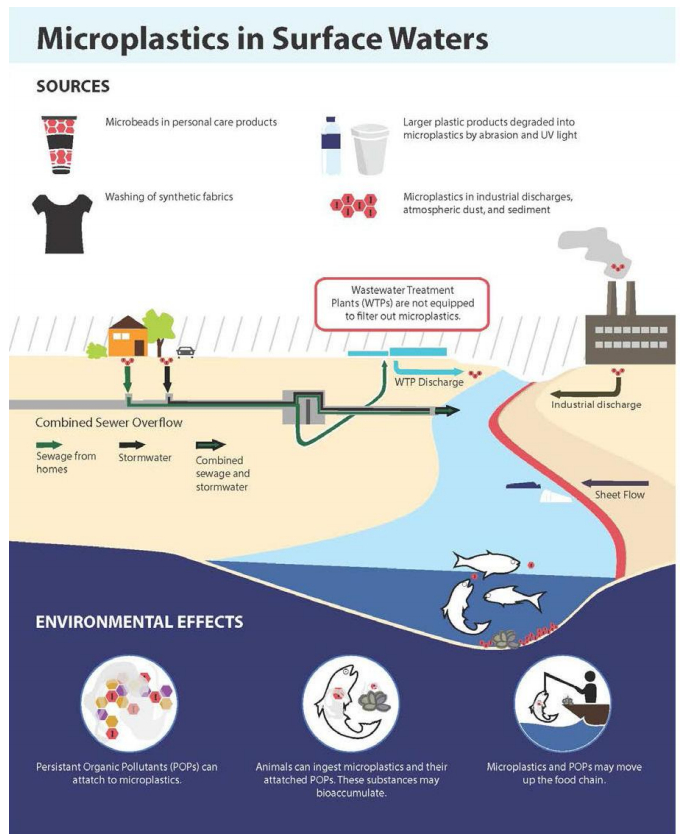 Figure 1. Sources, transport, and potential bioaccumulation of microplastics associated persistent organic compounds (POPs) released into the environment.
The goals of this study were to determine whether urban New Jersey freshwaters contained microplastic pollutants, and if so, to test analytic techniques that could potentially identify chemical compounds associated with this pollution. A third objective was to test whether identified associated compounds might have physiological effects on an aquatic organism. In order to assess potential effects associated with microplastic pollution in urban New Jersey (NJ) surface waters, we collected water samples and quantified microplastic densities, identified potential environmental breakdown products associated with three types of recovered microplastics, identified potentially mobile adsorbed organic compounds associated with the recovered microplastic particles, and exposed embryonic zebrafish to field recovered and pure microplastic samples.
Three replicate surface water samples were collected at each sampling location (N = 45) between May 12 and August 6,2016 (Table 1, Figure 2) to determine: (1) microplastic densities, (2) adsorbed compounds and plastic polymer composition(s), and (3) for toxicity testing. The Raritan and Passaic River watersheds were selected because they encompass some of the most densely developed urban and suburban areas in NJ, containing both residential and industrial properties. There are numerous permitted point sources discharging into both rivers within a 5-mile radius of the sampling locations, including personal care product producers, companies with "plastic" in their name, and wastewater treatment plants (Figure 2).
| Municipality | North | West | River |
| Sayreville | 40.47429 | –74.3574 | Raritan |
| Edison | 40.48746 | –74.3840 | Raritan |
| New Brunswick | 40.48884 | –74.4335 | Raritan |
| Piscataway | 40.54078 | –74.5124 | Raritan |
| Bridgewater | 40.54995 | –74.6687 | Raritan |
| Newark | 40.7129 | –74.119 | Passaic |
| Newark | 40.7333 | –74.1521 | Passaic |
| Kearny | 40.76401 | –74.1590 | Passaic |
| Lyndhurst | 40.8180 | –74.1350 | Passaic |
| Rutherford | 40.8300 | –74.1211 | Passaic |
| Elmwood Park | 40.9096 | –74.1320 | Passaic |
| Fairfield | 40.8979 | –74.2800 | Passaic |
| Livingston | 40.77899 | –74.3689 | Passaic |
| Chatham | 40.7387 | –74.3720 | Passaic |
| Berkeley Hts. | 40.6897 | –74.4390 | Passaic |
 DownLoad: CSV
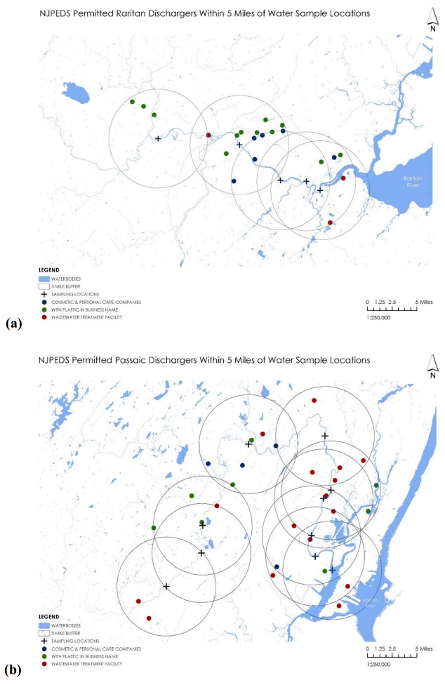 Figure 2. Map of (a) Raritan and (b) Passaic River Watershed. Sampling sites signified by black +. Location of facilities within a 5 mi. radius of the sampling site that have NJPEDs discharge permits issued by the State of New Jersey identified by blue (personal care companies), green (companies with "plastic" in their name, and red (waste water treatment plants) dots.
The Raritan River watershed is the largest contained within NJ, draining approximately 2862 km2 (see [33,34] for watershed descriptions pre-and post-urbanization, respectively). Samples were collected upriver (Bridgewater) and downriver of the North Branch/Lamington River, Millstone, and South Branch confluences (Piscataway, New Brunswick, Edison, Sayreville). The Passaic River Basin, home to over 2 million residents, is the third largest drainage basin within NJ, encompassing 2460 km2 [35]. Samples were collected under dry weather conditions (defined as a period without rain for at least 48 hours). Five Passaic River locations were also sampled under wet weather conditions (24 hours or less after a rain event of 2.2 cm). Sample collection from the urbanized lower river tidal reaches was conducted on an outgoing tide.
Water samples were collected using a manta trawl with attached flow meter (Model 315, OceanTest, Inc.). Accurate flow calculation is critical because flow rate determines the water volume used to calculate microplastic density. Due to low flow conditions outside the 0.20 m sec–1 accuracy range of the attached meter, flow was measured using a second flow meter (Marsh McBirney Flomatic Model 2000A) placed just downstream of the manta trawl net. Samples were collected through a rectangular opening 16 cm high × 61 cm wide, attached to a 333 μm mesh collection net 3 m long and 30 × 10 cm2 [19]. The net was held perpendicular to the current flow at the surface for 15 min. Flow distance was calculated using the attached flow meter count multiplied by the Impellor Constant (a factor of 0.245); the flow measurement from the second meter was read from the Marsh McBirney screen. Flow rates were compared using a Regression Analysis, which yielded an R2 of 0.89 (Figure 3). In order to compare sampling locations, we converted all attached flow meter values using Equation 1:
| FlowRate=(Attachedflowmeterdistance+160.62)/1.4201 | (1) |
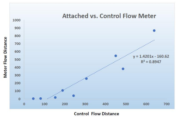 Figure 3. Regression analysis showing relationship of attached flow meter distance calculation versus hand held control meter distance.
After sample collection, the outside of the net was washed down with filtered site water to force collected material into a cod piece attached to the end of the trawl net, and the cod piece sample transferred to a glass collection jar. Isopropyl alcohol was added to one of the 3 replicates as a preservative; the other 2 samples were placed on ice for transport back to the laboratory.
Following protocols of Ericson et al. [19], one of each replicate sample was digested using the Fenton Reaction (20 mL of 0.05 M iron sulfate and 20 mL 30% hydrogen peroxide) to remove remaining organic material. Large organic particles were rinsed with DI to collect any attached plastic particles and the organic material discarded. To verify efficiency of microplastic recovery, 10 blue microbeads (0.330 mm diameter) were added to the Passaic samples. Reagent additions were repeated until the solution turned a pale yellow color and visible remnants of organic material were completely oxidized. This reaction does not digest the plastic particles. Recovered microplastics were placed under a dissecting microscope and separated into one of three size categories (0.355–0.999 mm, 1–4.749 mm, > 4.75 mm), and the type of plastic (fragment, pellet, fiber, film, or foam) within each size category determined. Total microplastic density was calculated using the formula:
| Plasticdensitykm−2=#microplasticsrecovered(netopeningxflowdistance) | (2) |
Different polymers exert various toxicities and adsorb other compounds in different quantities, and so knowledge of polymer composition is important in a microplastic environmental risk assessment. In a novel method of pyrolysis GC-MS, a very small piece of microplastic sample less than 1 mg in size was placed in a narrow quartz tube, which was then placed in a platinum coil and heated to 750 ℃. The intense heat breaks down large polymer chains into smaller fragments that are then analyzed by GS/MS to identify specific compounds. The fragmentation patterns have been reported to be reproducible and unique to a given polymer type [36]. Pure plastic samples (polyethylene high density, medium density and low density (HD, MD, and LD, respectively), polyethylene-co-vinyl acetate, polystyrene, polystyrene-co-acrylonitrile, polyvinylchloride, poly-methyl-methacrylate, sodium polyacrylate, polyurethane, polyethylene terephthalate, and polyamide) were purchased from Sigma Aldrich and analyzed by pyrolysis coupled with gas chromatography (Pyr-GC/MS) to create a "fingerprint" for comparison with three field collected microplastic samples (Figure 4).
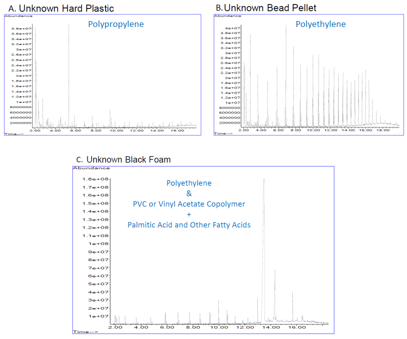 Figure 4. Identification of field collected plastic sample composition based upon analytical pyrolysis coupled with GC/MS. Mass spectra of (a) unknown hard plastic fragment indicates polypropylene composition; (b) unknown plastic bead pellet indicates polyethylene composition; and (c) unknown black foam indicates polyethylene and either PVC or vinyl acetate copolymer plus fatty acids.
To determine the presence of organic compounds sorbed to the microplastic particles, headspace solid phase micro extraction coupled with gas chromatography/ion trap mass spectrometry (HS-SPME/GC-ITMS) was employed. Microplastic solids and overlying site water were processed for organic contaminant analysis using A CTC Analytics Combi PAL system with SPME agitator attachment (Zwingen, Switzerland). This system combines headspace extraction of organics and injection. The Combi PAL HS-SPME and injection program run was: extraction time of 30 min. at 55 ℃ (water samples) or 75 ℃ (solid plastics), followed by pre-incubation time of 2.58 min., agitation speed of 350 rpm, agitation for 5 sec., agitation off for 2 sec., SPME fiber vial penetration of 25.0 mm, desorption time of 10 min., and injection penetration of 54.0 mm at 290 ℃ into a septum programmable injector (Varian 1079) operated in the splitless mode. Pre-and post-each sample injection, control blank runs with the SPME fiber (60 µm polydimethylsiloxane/divinylbenzene StableFlex fiber, Supelco, Bellefonte, PA, USA) were performed according to manufacturer instructions.
A Varian CP-3800 gas chromatography system (Walnut Creek, CA) equipped with A DBXLB 30 m column with a 0.18 mm ID and 0.18 μm film thickness (Agilent Technologies, Santa Clara, CA, USA) was used for chromatographic separation. Helium carrier gas flow was constantly maintained at 0.9 mL/min. Analyte elution from the GC column occurred using a temperature program that ranged from 35 ℃ to 320 ℃ over 40 min. Eluted compounds were analyzed by a Saturn 2200 ion trap mass spectrometer (Walnut Creek, CA), operated in EI positive mode and tuned with perfluorotributlyamine (FC-43) according to manufacturer's instructions. The electron multiplier voltage, emission current, multiplier offset, and modulation amplitude were set at 1750 V, 40 μA, +/–100, and 7.5 V, respectively. The ion trap was set at 225 ℃ and the transfer line at 275 ℃. Saturn GC/MS workstation (version 6.6 software) was used for data acquisition and integration. After background subtraction, unknown peaks were qualitatively identified by spectra comparison to the vendor's library and NIST/EPA/NIH 2012 mass spectral library. Identified compounds showing a correlation of > 70% fit to the library spectrum were defined as Tentatively Identified Compounds (TICs).
Recovered Fenton treated microplastics and pure polymers found in three microplastic field samples, identified using Pyr-GC/MS, were used in the larval fish experiments. The three samples (bead, pellet, and foam) were composed of polyethylene, polypropylene, and polyethylene-vinyl acetate copolymer, respectively (Figure 4). Larger particles of these pure plastics (Sigma Aldrich) and Fenton treated unknown plastics from a previously acquired field sample were pulverized using a dremel with a diamond tip followed by glass homogenization in 95% ethanol. The slurry was poured through a U.S.A Standard testing 2 mm sieve #10 (Fisher Scientific). The filtrate was collected and centrifuged in 95% ethanol for 15 min. at 8000 rpm. The supernatant was discarded and the pellet was completely dried by air pump for 24 hr. The dried pulverized plastic was weighed and re-suspended in autoclaved and aerated egg water to make microplastic concentrations of 1 or 10 μg/mL.
All fish studies were carried out using an approved IACUC approved protocol 08-025. AB strain zebrafish (Danio rerio) embryos were exposed to one type of microplastic per embryo at 3 hours post fertilization (hpf) and sacrificed at 96 hpf. Twenty embryos were randomly placed in individual glass vials and treated with 1.0 μg/mL or 10.0 μg/mL concentrations of pure microplastic. Autoclaved aerated egg-water was used as a control. Embryos were also exposed to field-collected microplastics in 1 or 10 μg/mL concentrations suspended in egg-water with methylene blue; controls were pure egg water and egg water with methylene blue. The embryos were incubated at 26 ℃ for 96 hpf in a static non-renewal protocol. Daily observations were made and observable lesions recorded. Upon endpoint of treatment, the sac fry were fixed in 10% buffered formalin and stained with Alcian Blue-Alizaran Red dye. Photographs and measurements (N = 20) were taken on an Olympus SZ-PT microscope with Scion camera and Adobe Photoshop CC 2015. Statistics were determined via Sigma Plot 11 software, used to calculate statistical significance with T tests and One Way ANOVA. Box plots were generated using the data and represent the mean plus and minus standard deviation with 75 and 25% boxes.
Microplastics, whose densities ranged from ~28,000 to over 3,000,000 particles km–2, were observed in all sampled locations (Figure 5); the types and quantities of microplastics were site specific (Tables 2 and 3). The most frequently recovered (38%) microplastic was fragment (broken off from a larger plastic item), followed by foam (breakdown of polystyrene items) > line (fiber, filament) > film (breakdown from bags, wrappers) > pellet (microbeads, nurdles). Recovered microplastic sizes were predominately (71%) in the larger 1 to > 4.5 mm size ranges. Passaic River densities were an order of magnitude greater than densities observed in the Raritan River (Figure 5; Table 2), which may be due to the population density in this highly urbanized watershed. The highest concentration of microplastics was observed during wet weather sampling (Figure 6). Raritan River microplastic density was highest at the two sites closest to Raritan Bay (Figures 2 and 5a). Conversely, downriver Passaic microplastic density was lower in the heavily urbanized locations (Figures 2 and 5b), although under wet weather conditions upriver Passaic densities decreased and the downriver Lyndhurst density increased (Figure 6).
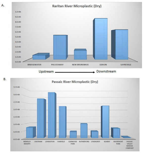 Figure 5. Microplastic densities (plastic units km–2) observed in (A. Raritan River and B. Passaic River) surface waters under dry weather conditions in summer, 2016.
| Location | Collection Conditions | Microplastic Type | Total | ||||
| Fragment | Pellet | Line | Film | Foam | |||
| Bridgewater | Dry | 6 | 0 | 1 | 0 | 0 | 7 |
| Piscataway | Dry | 0 | 8 | 9 | 23 | 0 | 40 |
| New Brunswick | Dry | 7 | 1 | 6 | 0 | 0 | 14 |
| Edison | Dry | 13 | 1 | 39 | 11 | 5 | 69 |
| Sayreville | Dry | 8 | 0 | 2 | 5 | 34 | 49 |
| Berkeley Heights | Dry | 31 | 0 | 4 | 3 | 14 | 52 |
| Berkeley Heights | Wet | 6 | 0 | 1 | 1 | 1 | 9 |
| Chatham | Dry | 163 | 16 | 206 | 33 | 65 | 483 |
| Chatham | Wet | 30 | 1 | 57 | 19 | 36 | 143 |
| Livingston | Dry | 94 | 3 | 56 | 22 | 54 | 229 |
| Livingston | Wet | 2 | 0 | 3 | 0 | 0 | 5 |
| Fairfield | Dry | 5 | 0 | 14 | 8 | 46 | 73 |
| Elmwood Park | Dry | 2 | 21 | 5 | 2 | 0 | 30 |
| Rutherford | Dry | 34 | 0 | 3 | 9 | 28 | 74 |
| Lyndhurst | Dry | 6 | 0 | 2 | 2 | 7 | 17 |
| Lyndhurst | Wet | 308 | 17 | 59 | 212 | 565 | 1161 |
| Kearny | Dry | 297 | 1 | 23 | 37 | 43 | 401 |
| Kearny | Wet | 176 | 3 | 3 | 11 | 32 | 225 |
| Newark | Dry | 14 | 2 | 4 | 14 | 21 | 55 |
| Newark | Dry | 1 | 0 | 1 | 0 | 1 | 3 |
| Total Recovered | 1203 | 74 | 498 | 412 | 952 | 3139 | |
| Total Recovered | 38.32% | 2.36% | 15.86% | 13.13% | 30.33% | ||
DownLoad: CSV| Location | Collection Conditions | Microplastic Type | Total | Recovery % | ||
| 0.3–0.99 mm | 1–4.75 mm | > 4.75 mm | ||||
| Bridgewater Raritan | Dry | 2 | 4 | 1 | 7 | N/A |
| Piscataway-Raritan | Dry | 16 | 15 | 9 | 40 | N/A |
| New Brunswick-Raritan | Dry | 5 | 9 | 0 | 14 | N/A |
| Edison-Raritan | Dry | 19 | 22 | 28 | 69 | N/A |
| Sayreville-Raritan | Dry | 7 | 30 | 12 | 49 | N/A |
| Berkeley Hts-Passaic | Dry | 24 | 25 | 3 | 52 | 100% |
| Berkeley Hts-Passaic | Wet | 0 | 7 | 2 | 9 | 10% |
| Chatham-Passaic | Dry | 167 | 207 | 109 | 483 | 100% |
| Chatham-Passaic | Wet | 22 | 65 | 56 | 143 | 80% |
| Livingston-Passaic | Dry | 128 | 77 | 24 | 229 | 20% |
| Livingston-Passaic | Wet | 0 | 3 | 2 | 5 | 40% |
| Fairfield-Passaic | Dry | 12 | 36 | 25 | 73 | N/A |
| Elmwood Park-Passaic | Dry | 30 | 0 | 0 | 30 | 100% |
| Rutherford-Passaic | Dry | 26 | 38 | 10 | 74 | 100% |
| Lyndhurst-Passaic | Dry | 3 | 8 | 6 | 17 | N/A |
| Lyndhurst-Passaic | Wet | 173 | 387 | 601 | 1161 | 60% |
| Kearny-Passaic | Dry | 165 | 188 | 48 | 401 | 80% |
| Kearny-Passaic | Wet | 97 | 113 | 15 | 225 | 50% |
| Newark-Passaic | Dry | 1 | 23 | 31 | 55 | 100% |
| Newark-Passaic | Dry | 2 | 1 | 0 | 3 | 60% |
| Total Recovered | 899 | 1258 | 982 | 3139 | ||
| % Total Recovered | 28.64% | 40.08% | 31.28% | |||
DownLoad: CSV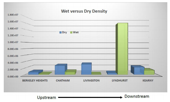 Figure 6. Microplastic densities (plastic units km–2) observed in surface waters from 5 Passaic River surface water sampling locations under dry and wet (<24 hrs. post rainfall) weather conditions in summer, 2016.
The HS-SPME GC/ITMS method allowed comparison of compounds identified/associated with the solid plastic particles, and demonstrates that the lower retention time compounds were also present in the water fraction (Figure 7). As shown, the TIC patterns observed for the different recovered microplastics have similar patterns to those of the pyrolysis coupled GC (Pyr-GC/MS) of pure plastic standards (Figure 8). In addition, individual peaks of interest can be further probed by examining the mass spectral flagged peaks of interest (Figure 8). Peaks with similar elution times and the same mass fragment patterns in both the solid plastic particles and in the water are strongly suggestive of plastic degradants/leachates contaminating the water. Using the fragmentation pattern, a library match can be determined as shown in Figure 9 for 2-Butanone, 4-(2, 6-trimethyl-1-cyclohexen-1yl.
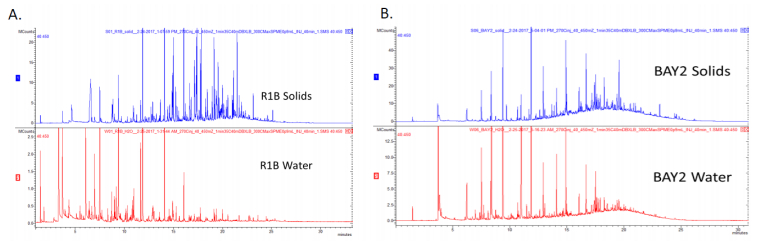 Figure 7. Comparison of GC/MS chromatograms from sample: (A) R1B solids and (B) Bay2 solids with the overlaying water from the collected field sample. The similarities between the early time points are lower molecular weight compounds either leaching out of, or desorbing from, non-Fenton reagent treated plastics in samples collected from the field. The later eluting peaks are not present in the water and represent the higher molecular weight compounds found in the plastics. Identification and confirmation is possible using library matches with the measured mass spectrum.
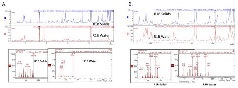 Figure 8. Comparison of 2 specific peaks having the same time retention (A) 11.6 min. and (B) 14.57 min.) and demonstrating comparable mass spectral fragmentation patterns.
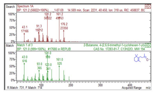 Figure 9. Library match of Spectrum 1A with 2-Butanone, 4-(2, 6-trimethyl-1-cyclohexen-1yl).
Exposure to the pure individual plastic compounds led to significant changes in zebrafish morphometrics. A significant increase in total body length was seen in polyethylene high density (HD) 10 μg/mL treatment exposure. Significant increase in the pericardial sack size was seen in polyethylene low density (LD) 10 μg/mL, polyethylene HD 1 μg/mL and 10 μg/mL, and polystyrene 1 μg/mL and 10 μg/mL treatment exposures (Figure 10). Conversely, exposure to microplastics recovered from the field samples after treatment with a Fenton reagent did not show any abnormalities (data not shown).
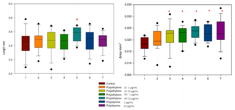 Figure 10. Embryonic fish in response to exposure to 3 plastic compounds in microplastic field samples and identified by PyGC. Red asterisk indicates p < 0.05.
This research demonstrates that microplastics are present in northern NJ surface waters, that POP are associated with these particles, and that these pollutants are mobile, found in both the water column and associated with the solid microplastics. Identical retention times for GC peaks found in both fractions indicated compounds can move between the two phases, making them potentially available for uptake by aquatic biota in the dissolved phase. Larval fish exhibited morphologic abnormalities when exposed to the polymers comprising microplastic fragment, bead, and foam particles recovered from the field samples. These abnormalities were not observed when the fish were exposed to microplastics that had been processed using the Fenton reagents that oxidize organic material. Our initial results indicate that lower molecular weight compounds are mobile, and may be carried in the water column beyond the location of the microplastic particles.
Using two methods (SPME GC/MS and Pyr-GC/MS) allows for the unambiguous identification of the compound(s) associated with microplastic debris and characterization of the major plastic type(s). By combining these two methods there is much greater confidence in identifying compounds that are derived from plastic versus non-plastic sources. In the future, specific "fingerprint" patterns can be used to categorize the class of plastics present in a waterbody and identify compounds that are associated with the particles. The GC/MS technique can be used for specific identification of compounds of environmental concern that are entering the waterway. This technique can also be used to identify compounds detected in biota that may be the result of ingesting or coming into contact with plastics or plastic-associated compounds. These analytical methods may be expanded into assessing pyrolysis of plastics and atmospheric contributions that are likely to occur when plastics are incinerated or sewage sludge contaminated with microplastics is used for energy production at sewage treatment facilities.
Density calculations, combined with identification of the polymer(s) and POPs associated with specific types of microplastic, can aide in calculating loadings of microplastic-associated pollution in a surface water body. The site specific amounts and types of plastic particles are potentially influenced by proximity to point source microplastic discharges, water flow rates, tributary connections, and river bathymetry. However, the data collected in these initial studies is not sufficient to identify specific pollution sources, and so further investigations that incorporate hydrologic flow patterns and bathymetry are needed.
Although previous samples (data not shown) indicate high microplastic densities in the NY/NJ harbor estuary, the heavily urbanized lower sections of the Passaic River did not exhibit the highest microplastic densities. This may be the result of tidally influenced flushing that dilutes plastic concentrations and moves the pollution out of the river and into the harbor. Tidal waters do not reach the Piscataway, Chatham, Livingston, or Fairfield upriver locations. The higher densities observed at these sites may be a function of the number of permitted discharges upriver of the sampling locations, inputs via tributary connections, or low flow conditions that allow plastics to accumulate. Because the downriver sites are tidally influenced, although samples were collected on outgoing tides it is possible that microplastic particles moved upriver from Newark (Lyndhurst, Kearny) or Raritan (Edison, Sayreville) Bays. Further research is needed to aide in microplastic source tracking.
Embryonic zebrafish exposed to plastic polymers identified by Pyr-GC/MS from field collected samples exhibited significant morphologic abnormalities (Figure 10). Field samples treated with the Fenton reagent did not result in alterations in growth or pericardial enlargement in the zebrafish embryos and yolk sac larvae. The Fenton reagent treatment, which oxidizes organic components and non-bound plasticizers, would leave only the polymerized plastic matrix. The plastic matrix scaffold would not be available for uptake into the embryo and likely explains the lack of toxic effects observed in these samples. This explanation is partially supported by the SPME-GCMS method, which demonstrated the same compounds on both the plastic particle and in the overlying water (Figures 7 and 8). Future studies will use both Fenton and non-Fenton treated samples, and will add exposure of juvenile fish, which would likely ingest the microplastic particles. The development of the analytical tools discussed above will enable us to determine the bioaccumulation of different compounds into aquatic organisms, both from the field and in laboratory studies.
There are a number of factors that make quantification of microplastic densities challenging [37]. In this study, density estimates could be affected by the limited number of samples, as well as temporal variations in microplastic inputs (i.e., post-precipitation sampling events, or conversely, drought conditions). Experimental bias may occur because the process for separating microplastics from organic material is labor intensive, and so there is the possibility of human error. Microbead spikes in the Passaic samples averaged 80% recovery, ranging from 20% (one sample) to 100% (5 samples), and so the density estimates may be understated. There is also potential experimental bias because the net mesh was 330 μm, and so smaller microplastics and any associated compounds are not captured in this dataset. In spite of these quantification challenges, our results demonstrate that there is a significant amount of microplastic in two of New Jersey's largest watersheds, and that potentially problematic organic compounds are associated with these particles.
This study demonstrates that urban New Jersey freshwaters contain microplastic pollutants that may have physiological effects on aquatic organisms. This proof of concept study demonstrates the ability to identify compounds associated with surface water microplastic pollution through a combination of SPME-GC and Pyr-GC/MS analytic methods. These methods can also determine which plastic-associated POPs are dissolved in the overlying water column. Once specific compounds are identified and microplastic densities are calculated, pollutant loadings, toxicological effects, and potential environmental risk can be assessed. These techniques may also be useful in identifying potential input sources based on the chemical "fingerprint" signatures of particle polymers and particle-associated compounds.
This work was carried out at the NJ Agricultural Experiment Station with funding support through Cooperative State Research, Education, and Extension Services Multi State 01201 and the National Institute of Environmental Health Sciences K99 ES025280. Funding for this research was also provided by the New Jersey Water Resources Research Institute FY2016 Program—Project ID 2016NJ378B (USGS Grant Award Number G16AP00071 and a grant from USEPA Urban Waters (EPA-OW-IO-15-01). We thank student interns Gabriella Bonaccorsi and Juan Carlos Ortega from East Side High School, Newark, NJ for their assistance with field sampling and laboratory analysis. We thank Anna Erickson and Angela Johnsen for providing assistance in preparing Figures.
The authors declare there is no conflict of interest.
| [1] |
Vollrath F, Porter D (2009) Silks as ancient models for modern polymers. Polymer 50: 5623–5632. doi: 10.1016/j.polymer.2009.09.068

|
| [2] | Lubec G, Holaubek J, Feldl C, et al. (1993) Use of silk in ancient Egypt. Nature 362: 25. |
| [3] |
Altman GH, Diaz F, Jakuba C, et al. (2003) Silk-based biomaterials. Biomaterials 24: 401–416. doi: 10.1016/S0142-9612(02)00353-8
|
| [4] |
Omenetto FG, Kaplan DL (2010) New opportunities for an ancient material. Science 329: 528–531. doi: 10.1126/science.1188936
|
| [5] |
Elices M, Plaza GR, Perez RJ, et al. (2011) The hidden link between supercontraction and mechanical behavior of spider silks. J Mech Behav Biomed Mater 4: 658–669. doi: 10.1016/j.jmbbm.2010.09.008
|
| [6] |
Cranford SW, Tarakanova A, Pugno NM, et al. (2012) Nonlinear material behaviour of spider silk yields robust webs. Nature 482: 72–76. doi: 10.1038/nature10739
|
| [7] |
Vollrath F, Porter D, Holland C (2013) The science of silks. MRS Bull 38: 73–80. doi: 10.1557/mrs.2012.314
|
| [8] |
Kluge JA, Rabotyagova O, Leisk GG, et al. (2008) Spider silks and their applications. Trends Biotechnol 26: 244–251. doi: 10.1016/j.tibtech.2008.02.006
|
| [9] |
Gatesy J, Hayashi C, Motriuk D, et al. (2001) Extreme diversity, conservation, and convergence of spider silk fibroin sequences. Science 291: 2603–2605. doi: 10.1126/science.1057561
|
| [10] |
Hardy JG, Scheibel TR (2009) Silk-inspired polymers and proteins. Biochem Soc T 37: 677–681. doi: 10.1042/BST0370677
|
| [11] |
Rising A, Johansson J (2015) Toward spinning artificial spider silk. Nat Chem Biol 11: 309–315. doi: 10.1038/nchembio.1789
|
| [12] |
Kim S, Marelli B, Brenckle MA, et al. (2014) All-water-based electron-beam lithography using silk as a resist. Nat Nanotechnol 9: 306–310. doi: 10.1038/nnano.2014.47
|
| [13] |
Omenetto FG, Kaplan DL (2008) A new route for silk. Nature Photonic 2: 641–643. doi: 10.1038/nphoton.2008.207
|
| [14] | Zhu B, Wang H, Leow WR, et al. (2016) Silk fibroin for flexible electronic devices. Adv Mater 22: 4250–4265. |
| [15] |
Doblhofer E, Schmid J, Riess M, et al. (2016) Structural insights into water-based spider silk protein-nanoclay composites with excellent gas and water vapor barrier properties. ACS Appl Mater Interface 8: 25535–25543. doi: 10.1021/acsami.6b08287
|
| [16] |
Marelli B, Brenckle MA, Kaplan DL, et al. (2016) Silk fibroin as edible coating for perishable food preservation. Sci Rep 6: 25263–25273. doi: 10.1038/srep25263
|
| [17] |
Abbott RD, Kimmerling EP, Cairns DM, et al. (2016) Silk as a biomaterial to support long-term three-dimensional tissue cultures. ACS Appl Mater Interface 8: 21861–21868. doi: 10.1021/acsami.5b12114
|
| [18] |
Jao D, Mou X, Hu X (2016) Tissue regeneration: a silk road. J Funct Biomater 7: 22–39. doi: 10.3390/jfb7030022
|
| [19] |
Kasoju N, Bora U (2012) Silk fibroin in tissue engineering. Adv Healthc Mater 1: 393–412. doi: 10.1002/adhm.201200097
|
| [20] |
Werner V, Meinel L (2015) From silk spinning in insects and spiders to advanced silk fibroin drug delivery systems. Eur J Pharm Biopharm 97: 392–399. doi: 10.1016/j.ejpb.2015.03.016
|
| [21] |
Yucel T, Lovett ML, Kaplan DL (2014) Silk-based biomaterials for sustained drug delivery. J Control Release 190: 381–397. doi: 10.1016/j.jconrel.2014.05.059
|
| [22] | Seib FP, Kaplan DL (2013) Silk for drug delivery applications: opportunities and challenges. Israel J Chem 53: 756–766. |
| [23] |
Thurber AE, Omenetto FG, Kaplan DL (2015) In vivo bioresponses to silk proteins. Biomaterials 71: 145–157. doi: 10.1016/j.biomaterials.2015.08.039
|
| [24] |
Pritchard EM, Dennis PB, Omenetto FG, et al. (2012) Physical and chemical aspects of stabilization of compounds in silk. Biopolymers 97: 479–498. doi: 10.1002/bip.22026
|
| [25] |
Chiu B, Coburn J, Pilichowska M, et al. (2014) Surgery combined with controlled-release doxorubicin silk films as a treatment strategy in an orthotopic neuroblastoma mouse model. Brit J Cancer 111: 708–715. doi: 10.1038/bjc.2014.324
|
| [26] |
Seib FP, Coburn J, Konrad I, et al. (2015) Focal therapy of neuroblastoma using silk films to deliver kinase and chemotherapeutic agents in vivo. Acta Biomater 20: 32–38. doi: 10.1016/j.actbio.2015.04.003
|
| [27] |
Coburn J, Harris J, Zakharov AD, et al. (2017) Implantable chemotherapy-loaded silk protein materials for neuroblastoma treatment. Int J Cancer 140: 726–735. doi: 10.1002/ijc.30479
|
| [28] |
Seib FP, Pritchard EM, Kaplan DL (2013) Self-assembling doxorubicin silk hydrogels for the focal treatment of primary breast cancer. Adv Funct Mater 23: 58–65. doi: 10.1002/adfm.201201238
|
| [29] |
Jastrzebska K, Kucharczyk K, Florczak A, et al. (2015) Silk as an innovative biomaterial for cancer therapy. Rep Pract Oncol Radiother 20: 87–98. doi: 10.1016/j.rpor.2014.11.010
|
| [30] | Coleman RE (2012) Bone cancer in 2011: prevention and treatment of bone metastases. Nat Rev Clin Oncol 9: 76–78. |
| [31] |
Gupta GP, Massague J (2006) Cancer metastasis: building a framework. Cell 127: 679–695. doi: 10.1016/j.cell.2006.11.001
|
| [32] |
Ehrlich P (1913) Address in pathology, on chemiotherapy: delivered before the seventeenth international congress of medicine. Brit Med J 2: 353–359. doi: 10.1136/bmj.2.2746.353
|
| [33] |
Mottaghitalab F, Farokhi M, Shokrgozar MA, et al. (2015) Silk fibroin nanoparticle as a novel drug delivery system. J Control Release 206: 161–176. doi: 10.1016/j.jconrel.2015.03.020
|
| [34] |
Zhao Z, Li Y, Xie MB (2015) Silk fibroin-based nanoparticles for drug delivery. Int J Mol Sci 16: 4880–4903. doi: 10.3390/ijms16034880
|
| [35] |
Ebrahimi D, Tokareva O, Rim NG, et al. (2015) Silk-its mysteries, how it is made, and how it is used. ACS Biomater Sci Eng 1: 864–876. doi: 10.1021/acsbiomaterials.5b00152
|
| [36] |
Eisoldt L, Thamm C, Scheibel T (2012) Review the role of terminal domains during storage and assembly of spider silk proteins. Biopolymers 97: 355–361. doi: 10.1002/bip.22006
|
| [37] | Xu G, Gong L, Yang Z, et al. (2014) What makes spider silk fibers so strong? From molecular-crystallite network to hierarchical network structures. Soft Mat 10: 2116–2123. |
| [38] |
Ha SW, Gracz HS, Tonelli AE, et al. (2005) Structural study of irregular amino acid sequences in the heavy chain of bombyx mori silk fibroin. Biomacromolecules 6: 2563–2569. doi: 10.1021/bm050294m
|
| [39] |
Asakura T, Ohgo K, Ishida T, et al. (2005) Possible implications of serine and tyrosine residues and intermolecular interactions on the appearance of silk istructure of bombyx mori silk fibroin-derived synthetic peptides: high-resolution 13c cross-polarization/magic-angle spinning NMR study. Biomacromolecules 6: 468–474. doi: 10.1021/bm049487k
|
| [40] |
Asakura T, Okushita K, Williamson MP (2015) Analysis of the structure of bombyx mori silk fibroin by NMR. Macromolecules 48: 2345–2357. doi: 10.1021/acs.macromol.5b00160
|
| [41] |
Zhou CZ, Confalonieri F, Jacquet M, et al. (2001) Silk fibroin: structural implications of a remarkable amino acid sequence. Proteins 44: 119–122. doi: 10.1002/prot.1078
|
| [42] |
Zhou CZ, Confalonieri F, Medina N, et al. (2000) Fine organization of bombyx mori fibroin heavy chain gene. Nucleic Acids Res 28: 2413–2419. doi: 10.1093/nar/28.12.2413
|
| [43] |
Jin HJ, Kaplan DL (2003) Mechanism of silk processing in insects and spiders. Nature 424: 1057–1061. doi: 10.1038/nature01809
|
| [44] |
Greving I, Dicko C, Terry A, et al. (2010) Small angle neutron scattering of native and reconstituted silk fibroin. Soft Mat 6: 4389–4395. doi: 10.1039/c0sm00108b
|
| [45] |
Lu Q, Zhu H, Zhang C, et al. (2012) Silk self-assembly mechanisms and control from thermodynamics to kinetics. Biomacromolecules 13: 826–832. doi: 10.1021/bm201731e
|
| [46] |
Wang X, Yucel T, Lu Q, et al. (2010) Silk nanospheres and microspheres from silk/pva blend films for drug delivery. Biomaterials 31: 1025–1035. doi: 10.1016/j.biomaterials.2009.11.002
|
| [47] |
Myung SJ, Kim HS, Kim Y, et al. (2008) Fluorescent silk fibroin nanoparticles prepared using a reverse microemulsion. Macromol Res 16: 604–608. doi: 10.1007/BF03218567
|
| [48] | Gupta V, Aseh A, Rios CN, et al. (2009) Fabrication and characterization of silk fibroin-derived curcumin nanoparticles for cancer therapy. Int J Nanomed 4: 115–122. |
| [49] |
Lammel AS, Hu X, Park SH, et al. (2010) Controlling silk fibroin particle features for drug delivery. Biomaterials 31: 4583–4591. doi: 10.1016/j.biomaterials.2010.02.024
|
| [50] |
Kundu J, Chung YI, Kim YH, et al. (2010) Silk fibroin nanoparticles for cellular uptake and control release. Int J Pharm 388: 242–250. doi: 10.1016/j.ijpharm.2009.12.052
|
| [51] |
Seib FP, Jones GT, Rnjak KJ, et al. (2013) pH-dependent anticancer drug release from silk nanoparticles. Adv Healthc Mater 2: 1606–1611. doi: 10.1002/adhm.201300034
|
| [52] | Wongpinyochit T, Johnston BF, Seib FP (2016) Manufacture and drug delivery applications of silk nanoparticles. J Vis Exp DOI: 10.3791/54669. |
| [53] |
Zhang YQ, Shen WD, Xiang RL, et al. (2007) Formation of silk fibroin nanoparticles in water-miscible organic solvent and their characterization. J Nanopart Res 9: 885–900. doi: 10.1007/s11051-006-9162-x
|
| [54] | Zhao Z, Xie M, Li Y, et al. (2015) Formation of curcumin nanoparticles via solution-enhanced dispersion by supercritical CO2. Int J Nanomed 10: 3171–3181. |
| [55] | Lozano PAA, Montalban MG, Aznar CSD, et al. (2015) Production of silk fibroin nanoparticles using ionic liquids and high-power ultrasounds. J Appl Polym Sci 132: 41702–41709. |
| [56] | Gholami A, Tavanai H, Moradi AR (2010) Production of fibroin nanopowder through electrospraying. J Nanopart Res 13: 2089–2098. |
| [57] |
Wenk E, Wandrey AJ, Merkle HP, et al. (2008) Silk fibroin spheres as a platform for controlled drug delivery. J Control Release 132: 26–34. doi: 10.1016/j.jconrel.2008.08.005
|
| [58] |
Lu Q, Huang Y, Li M, et al. (2011) Silk fibroin electrogelation mechanisms. Acta Biomater 7: 2394–2400. doi: 10.1016/j.actbio.2011.02.032
|
| [59] |
Rajkhowa R, Wang L, Wang X (2008) Ultra-fine silk powder preparation through rotary and ball milling. Powder Technol 185: 87–95. doi: 10.1016/j.powtec.2008.01.005
|
| [60] |
Mathur AB, Gupta V (2010) Silk fibroin-derived nanoparticles for biomedical applications. Nanomedicine 5: 807–820. doi: 10.2217/nnm.10.51
|
| [61] |
Xiao L, Lu G, Lu Q, et al. (2016) Direct formation of silk nanoparticles for drug delivery. ACS Biomater Sci Eng 2: 2050–2057. doi: 10.1021/acsbiomaterials.6b00457
|
| [62] |
Wongpinyochit T, Uhlmann P, Urquhart AJ, et al. (2015) PEGylated silk nanoparticles for anticancer drug delivery. Biomacromolecules 16: 3712–3722. doi: 10.1021/acs.biomac.5b01003
|
| [63] |
Subia B, Chandra S, Talukdar S, et al. (2014) Folate conjugated silk fibroin nanocarriers for targeted drug delivery. Integr Biol 6: 203–214. doi: 10.1039/C3IB40184G
|
| [64] |
Rabanel JM, Hildgen P, Banquy X (2014) Assessment of PEG on polymeric particles surface, a key step in drug carrier translation. J Control Release 185: 71–87. doi: 10.1016/j.jconrel.2014.04.017
|
| [65] |
Pasut G, Veronese FM (2012) State of the art in PEGylation: the great versatility achieved after forty years of research. J Control Release 161: 461–472. doi: 10.1016/j.jconrel.2011.10.037
|
| [66] |
Wang S, Xu T, Yang Y, et al. (2015) Colloidal stability of silk fibroin nanoparticles coated with cationic polymer for effective drug delivery. ACS Appl Mater Interface 7: 21254–21262. doi: 10.1021/acsami.5b05335
|
| [67] |
Tian Y, Jiang X, Chen X, et al. (2014) Doxorubicin-loaded magnetic silk fibroin nanoparticles for targeted therapy of multidrug-resistant cancer. Adv Mater 26: 7393–7398. doi: 10.1002/adma.201403562
|
| [68] |
Chung H, Kim TY, Lee SY (2012) Recent advances in production of recombinant spider silk proteins. Curr Opin Biotech 23: 957–964. doi: 10.1016/j.copbio.2012.03.013
|
| [69] |
Lammel A, Schwab M, Hofer M, et al. (2011) Recombinant spider silk particles as drug delivery vehicles. Biomaterials 32: 2233–2240. doi: 10.1016/j.biomaterials.2010.11.060
|
| [70] |
Humenik M, Smith AM, Scheibel T (2011) Recombinant spider silks-biopolymers with potential for future applications. Polymers 3: 640–661. doi: 10.3390/polym3010640
|
| [71] |
Schierling MB, Doblhofer E, Scheibel T (2016) Cellular uptake of drug loaded spider silk particles. Biomater Sci 4: 1515–1523. doi: 10.1039/C6BM00435K
|
| [72] |
Doblhofer E, Scheibel T (2015) Engineering of recombinant spider silk proteins allows defined uptake and release of substances. J Pharm Sci 104: 988–994. doi: 10.1002/jps.24300
|
| [73] |
Elsner MB, Herold HM, Muller HS, et al. (2015) Enhanced cellular uptake of engineered spider silk particles. Biomater Sci 3: 543–551. doi: 10.1039/C4BM00401A
|
| [74] |
Florczak A, Mackiewicz A, Dams KH (2014) Functionalized spider silk spheres as drug carriers for targeted cancer therapy. Biomacromolecules 15: 2971–2981. doi: 10.1021/bm500591p
|
| [75] |
Neubauer MP, Blüm C, Agostini E, et al. (2013) Micromechanical characterization of spider silk particles. Biomater Sci 1: 1160–1165. doi: 10.1039/c3bm60108k
|
| [76] |
Anselmo AC, Zhang M, Kumar S, et al. (2015) Elasticity of nanoparticles influences their blood circulation, phagocytosis, endocytosis, and targeting. ACS Nano 9: 3169–3177. doi: 10.1021/acsnano.5b00147
|
| [77] |
Numata K, Kaplan DL (2010) Silk-based delivery systems of bioactive molecules. Adv Drug Deliver Rev 62: 1497–1508. doi: 10.1016/j.addr.2010.03.009
|
| [78] |
Numata K, Subramanian B, Currie HA, et al. (2009) Bioengineered silk protein-based gene delivery systems. Biomaterials 30: 5775–5784. doi: 10.1016/j.biomaterials.2009.06.028
|
| [79] |
Numata K, Hamasaki J, Subramanian B, et al. (2010) Gene delivery mediated by recombinant silk proteins containing cationic and cell binding motifs. J Control Release 146: 136–143. doi: 10.1016/j.jconrel.2010.05.006
|
| [80] |
Numata K, Kaplan DL (2010) Silk-based gene carriers with cell membrane destabilizing peptides. Biomacromolecules 11: 3189–3195. doi: 10.1021/bm101055m
|
| [81] |
Numata K, Reagan MR, Goldstein RH, et al. (2011) Spider silk-based gene carriers for tumor cell-specific delivery. Bioconjugate Chem 22: 1605–1610. doi: 10.1021/bc200170u
|
| [82] |
Seib FP, Herklotz M, Burke KA, et al. (2014) Multifunctional silk-heparin biomaterials for vascular tissue engineering applications. Biomaterials 35: 83–91. doi: 10.1016/j.biomaterials.2013.09.053
|
| [83] |
Seib FP, Maitz MF, Hu X, et al. (2012) Impact of processing parameters on the haemocompatibility of bombyx mori silk films. Biomaterials 33: 1017–1023. doi: 10.1016/j.biomaterials.2011.10.063
|
| [84] |
Murphy AR, Kaplan DL (2009) Biomedical applications of chemically-modified silk fibroin. J Mater Chem 19: 6443–6450. doi: 10.1039/b905802h
|
| [85] |
Kambe Y, Yamamoto K, Kojima K, et al. (2010) Effects of RGDS sequence genetically interfused in the silk fibroin light chain protein on chondrocyte adhesion and cartilage synthesis. Biomaterials 31: 7503–7511. doi: 10.1016/j.biomaterials.2010.06.045
|
| [86] |
Teule F, Miao YG, Sohn BH, et al. (2012) Silkworms transformed with chimeric silkworm/spider silk genes spin composite silk fibers with improved mechanical properties. P Natl Acad Sci USA 109: 923–928. doi: 10.1073/pnas.1109420109
|
| [87] |
Xia XX, Qian ZG, Ki CS, et al. (2010) Native-sized recombinant spider silk protein produced in metabolically engineered Escherichia coli results in a strong fiber. P Natl Acad Sci USA 107: 14059–14063. doi: 10.1073/pnas.1003366107
|
| [88] | Wray LS, Hu X, Gallego J, et al. (2011) Effect of processing on silk-based biomaterials: reproducibility and biocompatibility. J Biomed Mater Res 99: 89–101. |
| [89] |
Rockwood DN, Preda RC, Yucel T, et al. (2011) Materials fabrication from bombyx mori silk fibroin. Nat Protoc 6: 1612–1631. doi: 10.1038/nprot.2011.379
|
| [90] |
Duncan R, Gaspar R (2011) Nanomedicine(s) under the microscope. Mol Pharm 8: 2101–2141. doi: 10.1021/mp200394t
|
| [91] |
Sheridan C (2012) Proof of concept for next-generation nanoparticle drugs in humans. Nature Biotechnol 30: 471–473. doi: 10.1038/nbt0612-471
|
| [92] | Shi J, Kantoff PW, Wooster R, et al. (2017) Cancer nanomedicine: progress, challenges and opportunities. Nat Rev Cancer 17: 20–37. |
| [93] |
Maeda H, Nakamura H, Fang J (2013) The EPR effect for macromolecular drug delivery to solid tumors: improvement of tumor uptake, lowering of systemic toxicity, and distinct tumor imaging in vivo. Adv Drug Deliver Rev 65: 71–79. doi: 10.1016/j.addr.2012.10.002
|
| [94] |
Duncan R (2006) Polymer conjugates as anticancer nanomedicines. Nat Rev Cancer 6: 688–701. doi: 10.1038/nrc1958
|
| [95] |
Juliano R (2013) Nanomedicine: is the wave cresting? Nat Rev Drug Discov 12: 171–172. doi: 10.1038/nrd3958
|
| [96] | Venditto VJ, Szoka FC (2013) Cancer nanomedicines: so many papers and so few drugs! Adv Drug Deliver Rev 65: 80–88. |
| [97] | Wilhelm S, Tavares AJ, Dai Q, et al. (2016) Analysis of nanoparticle delivery to tumours. Nature Rev Mater 1: 1–12. |
| [98] |
Cleal K, He L, Watson PD, et al. (2013) Endocytosis, intracellular traffic and fate of cell penetrating peptide based conjugates and nanoparticles. Curr Pharm Design 19: 2878–2894. doi: 10.2174/13816128113199990297
|
| [99] |
Duncan R, Richardson SC (2012) Endocytosis and intracellular trafficking as gateways for nanomedicine delivery: opportunities and challenges. Mol Pharm 9: 2380–2402. doi: 10.1021/mp300293n
|
| [100] |
Whitehead KA, Langer R, Anderson DG (2009) Knocking down barriers: advances in siRNA delivery. Nat Rev Drug Discov 8: 129–138. doi: 10.1038/nrd2742
|
| [101] |
Gratton SE, Ropp PA, Pohlhaus PD, et al. (2008) The effect of particle design on cellular internalization pathways. P Natl Acad Sci USA 105: 11613–11618. doi: 10.1073/pnas.0801763105
|
| [102] |
Herd H, Daum N, Jones AT, et al. (2013) Nanoparticle geometry and surface orientation influence mode of cellular uptake. ACS Nano 7: 1961–1973. doi: 10.1021/nn304439f
|
| [103] |
Rejman J, Oberle V, Zuhorn IS, et al. (2004) Size-dependent internalization of particles via the pathways of clathrin- and caveolae-mediated endocytosis. Biochem J 377: 159–169. doi: 10.1042/bj20031253
|
| [104] |
Oh P, Borgstrom P, Witkiewicz H, et al. (2007) Live dynamic imaging of caveolae pumping targeted antibody rapidly and specifically across endothelium in the lung. Nat Biotechnol 25: 327–337. doi: 10.1038/nbt1292
|
| [105] |
Sabharanjak S, Mayor S (2004) Folate receptor endocytosis and trafficking. Adv Drug Deliver Rev 56: 1099–1109. doi: 10.1016/j.addr.2004.01.010
|
| [106] |
Mosesson Y, Mills GB, Yarden Y (2008) Derailed endocytosis: an emerging feature of cancer. Nat Rev Cancer 8: 835–850. doi: 10.1038/nrc2521
|
| [107] |
Vercauteren D, Vandenbroucke RE, Jones AT, et al. (2010) The use of inhibitors to study endocytic pathways of gene carriers: optimization and pitfalls. Mol Ther 18: 561–569. doi: 10.1038/mt.2009.281
|
| 1. | Malin Klein, Elke K. Fischer, Microplastic abundance in atmospheric deposition within the Metropolitan area of Hamburg, Germany, 2019, 685, 00489697, 96, 10.1016/j.scitotenv.2019.05.405 | |
| 2. | Guanjun Xu, Hanyun Cheng, Robin Jones, Yiqing Feng, Kedong Gong, Kejian Li, Xiaozhong Fang, Muhammad Ali Tahir, Ventsislav Kolev Valev, Liwu Zhang, Surface-Enhanced Raman Spectroscopy Facilitates the Detection of Microplastics <1 μm in the Environment, 2020, 54, 0013-936X, 15594, 10.1021/acs.est.0c02317 | |
| 3. | Jangsun Hwang, Daheui Choi, Seora Han, Se Yong Jung, Jonghoon Choi, Jinkee Hong, Potential toxicity of polystyrene microplastic particles, 2020, 10, 2045-2322, 10.1038/s41598-020-64464-9 | |
| 4. | Susanne M. Brander, Violet C. Renick, Melissa M. Foley, Clare Steele, Mary Woo, Amy Lusher, Steve Carr, Paul Helm, Carolynn Box, Sam Cherniak, Robert C. Andrews, Chelsea M. Rochman, Sampling and Quality Assurance and Quality Control: A Guide for Scientists Investigating the Occurrence of Microplastics Across Matrices, 2020, 74, 0003-7028, 1099, 10.1177/0003702820945713 | |
| 5. | Quinn T. Birch, Phillip M. Potter, Patricio X. Pinto, Dionysios D. Dionysiou, Souhail R. Al-Abed, Sources, transport, measurement and impact of nano and microplastics in urban watersheds, 2020, 19, 1569-1705, 275, 10.1007/s11157-020-09529-x | |
| 6. | Tanja Kögel, Ørjan Bjorøy, Benuarda Toto, André Marcel Bienfait, Monica Sanden, Micro- and nanoplastic toxicity on aquatic life: Determining factors, 2020, 709, 00489697, 136050, 10.1016/j.scitotenv.2019.136050 | |
| 7. | Marlon Ferraz, Amanda Leticia Bauer, Victor Hugo Valiati, Uwe Horst Schulz, Microplastic Concentrations in Raw and Drinking Water in the Sinos River, Southern Brazil, 2020, 12, 2073-4441, 3115, 10.3390/w12113115 | |
| 8. | Muhammad Irfan, Abdul Qadir, Mehvish Mumtaz, Sajid Rashid Ahmad, An unintended challenge of microplastic pollution in the urban surface water system of Lahore, Pakistan, 2020, 27, 0944-1344, 16718, 10.1007/s11356-020-08114-7 | |
| 9. | Fatima Zohra Benouis, Ould Amer Yacine, Heat Transfer Enhancement of Heat Sources at its Optimum Position in a Square Enclosure with Ventilation Ports, 2021, 406, 1662-9507, 12, 10.4028/www.scientific.net/DDF.406.12 | |
| 10. | Peter Kusch, 2020, Chapter 41-1, 978-3-030-10618-8, 1, 10.1007/978-3-030-10618-8_41-1 | |
| 11. | Rong Qiu, Yang Song, Xiaoting Zhang, Bing Xie, Defu He, 2020, Chapter 447, 978-3-030-56270-0, 41, 10.1007/698_2020_447 | |
| 12. | Christian Dunn, Jedd Owens, Luke Fears, Laura Nunnerley, Julian Kirby, Oliver L. Armstrong, P. John Thomas, Dan Aberg, William Gilder, Dannielle Green, Rachael Antwis, Chris Freeman, An affordable methodology for quantifying waterborne microplastics - an emerging contaminant in inland-waters, 2019, 79, 1723-8633, 10.4081/jlimnol.2019.1943 | |
| 13. | B. Ravit, K. Cooper, B. Buckley, I. Yang, A. Deshpande, Organic compounds associated with microplastic pollutants in New Jersey, U.S.A. surface waters, 2019, 6, 2372-0352, 445, 10.3934/environsci.2019.6.445 | |
| 14. | Nora Expósito, Joaquim Rovira, Jordi Sierra, Jaume Folch, Marta Schuhmacher, Microplastics levels, size, morphology and composition in marine water, sediments and sand beaches. Case study of Tarragona coast (western Mediterranean), 2021, 786, 00489697, 147453, 10.1016/j.scitotenv.2021.147453 | |
| 15. | Karli Sipps, Georgia Arbuckle-Keil, Robert Chant, Nicole Fahrenfeld, Lori Garzio, Kasey Walsh, Grace Saba, Pervasive occurrence of microplastics in Hudson-Raritan estuary zooplankton, 2022, 817, 00489697, 152812, 10.1016/j.scitotenv.2021.152812 | |
| 16. | Jasmine T. Yu, Miriam L. Diamond, Paul A. Helm, A fit‐for‐purpose categorization scheme for microplastic morphologies, 2023, 19, 1551-3777, 422, 10.1002/ieam.4648 | |
| 17. | Sechul Chun, Manikandan Muthu, Judy Gopal, Mass Spectrometry as an Analytical Tool for Detection of Microplastics in the Environment, 2022, 10, 2227-9040, 530, 10.3390/chemosensors10120530 | |
| 18. | Quinn T. Birch, Phillip M. Potter, Patricio X. Pinto, Dionysios D. Dionysiou, Souhail R. Al-Abed, Isotope ratio mass spectrometry and spectroscopic techniques for microplastics characterization, 2021, 224, 00399140, 121743, 10.1016/j.talanta.2020.121743 | |
| 19. | Gina M. Moreno, Keith R. Cooper, Morphometric effects of various weathered and virgin/pure microplastics on sac fry zebrafish (Danio rerio), 2021, 8, 2372-0352, 204, 10.3934/environsci.2021014 | |
| 20. | Ida Florance, Seenivasan Ramasubbu, Amitava Mukherjee, Natarajan Chandrasekaran, Polystyrene nanoplastics dysregulate lipid metabolism in murine macrophages in vitro, 2021, 458, 0300483X, 152850, 10.1016/j.tox.2021.152850 | |
| 21. | Shama E. Haque, 2022, 6, 9780323918381, 21, 10.1016/B978-0-323-91838-1.00001-4 | |
| 22. | Peter Kusch, 2022, Chapter 41, 978-3-030-39040-2, 477, 10.1007/978-3-030-39041-9_41 | |
| 23. | Maria Cristina Guerrera, Marialuisa Aragona, Caterina Porcino, Francesco Fazio, Rosaria Laurà, Maria Levanti, Giuseppe Montalbano, Germana Germanà, Francesco Abbate, Antonino Germanà, Micro and Nano Plastics Distribution in Fish as Model Organisms: Histopathology, Blood Response and Bioaccumulation in Different Organs, 2021, 11, 2076-3417, 5768, 10.3390/app11135768 | |
| 24. | Ya-Qi Zhang, Marianna Lykaki, Mohammad Taher Alrajoula, Marta Markiewicz, Caroline Kraas, Sabrina Kolbe, Kristina Klinkhammer, Maike Rabe, Robert Klauer, Ellen Bendt, Stefan Stolte, Microplastics from textile origin – emission and reduction measures, 2021, 23, 1463-9262, 5247, 10.1039/D1GC01589C | |
| 25. | Diana Nantege, Robinson Odong, Helen Shnada Auta, Unique Ndubuisi Keke, Gilbert Ndatimana, Attobla Fulbert Assie, Francis Ofurum Arimoro, Microplastic pollution in riverine ecosystems: threats posed on macroinvertebrates, 2023, 1614-7499, 10.1007/s11356-023-27839-9 | |
| 26. | Scott Douglas, Genevieve Clifton, Joselyn Wall, Kelly Rosofsky, Christopher Mullan, Recovery of the NJ marine transportation system in the wake of Superstorm Sandy: A 10-year retrospective, 2023, 2641-7286, 55, 10.34237/1009147 | |
| 27. | S. Mustapha, J.O. Tijani, R. Elabor, R.B. Salau, T.C. Egbosiuba, A.T. Amigun, D.T. Shuaib, A. Sumaila, T. Fiola, Y.K. Abubakar, H.L. Abubakar, I.F. Ossamulu, S.A. Abdulkareem, M.M. Ndamitso, S. Sagadevan, A.K. Mohammed, Technological approaches for removal of microplastics and nanoplastics in the environment, 2024, 22133437, 112084, 10.1016/j.jece.2024.112084 | |
| 28. | Fengyang Hu, Yajie Cai, Lingliang Kong, Min Zhou, Dafa Sun, Xue Guo, Wei Li, Yongzhai Mai, Xuesong Wang, Effects of polystyrene nanoplastics on the amino acid composition of Asian Clam (Corbicula fluminea), 2024, 198, 00236438, 115998, 10.1016/j.lwt.2024.115998 | |
| 29. | Farzaneh Feizi, Razegheh Akhbarizadeh, Amir Hossein Hamidian, Microplastics in urban water systems, Tehran Metropolitan, Iran, 2024, 196, 0167-6369, 10.1007/s10661-024-12815-8 | |
| 30. | Salam Suresh Singh, Rajdeep Chanda, Ngangbam Somen Singh, Ningthoujam Ranjana Devi, Khoisnam Vramari Devi, Keshav Kumar Upadhyay, S. K. Tripathi, Microplastic pollution: exploring trophic transfer pathways and ecological impacts, 2024, 2, 2731-9431, 10.1007/s44274-024-00139-w | |
| 31. | Caglar Berkel, Oguz Özbek, Methods used in the identification and quantification of micro(nano)plastics from water environments, 2024, 10269185, 10.1016/j.sajce.2024.09.010 | |
| 32. | Stanley Chukwuemeka Ihenetu, Christian Ebere Enyoh, Chunhui Wang, Gang Li, Sustainable Urbanization and Microplastic Management: Implications for Human Health and the Environment, 2024, 8, 2413-8851, 252, 10.3390/urbansci8040252 | |
| 33. | Collins Nana Andoh, Peter Donkor, John Aboagye, Ghana's environmental law and waterbody protection: A critical assessment of plastic pollution regulations, 2025, 380, 03014797, 125172, 10.1016/j.jenvman.2025.125172 |
Figures(5)

F. Philipp Seib. Silk nanoparticles—an emerging anticancer nanomedicine[J]. AIMS Bioengineering, 2017, 4(2): 239-258. doi: 10.3934/bioeng.2017.2.239

| Municipality | North | West | River |
| Sayreville | 40.47429 | –74.3574 | Raritan |
| Edison | 40.48746 | –74.3840 | Raritan |
| New Brunswick | 40.48884 | –74.4335 | Raritan |
| Piscataway | 40.54078 | –74.5124 | Raritan |
| Bridgewater | 40.54995 | –74.6687 | Raritan |
| Newark | 40.7129 | –74.119 | Passaic |
| Newark | 40.7333 | –74.1521 | Passaic |
| Kearny | 40.76401 | –74.1590 | Passaic |
| Lyndhurst | 40.8180 | –74.1350 | Passaic |
| Rutherford | 40.8300 | –74.1211 | Passaic |
| Elmwood Park | 40.9096 | –74.1320 | Passaic |
| Fairfield | 40.8979 | –74.2800 | Passaic |
| Livingston | 40.77899 | –74.3689 | Passaic |
| Chatham | 40.7387 | –74.3720 | Passaic |
| Berkeley Hts. | 40.6897 | –74.4390 | Passaic |
DownLoad: CSV| Location | Collection Conditions | Microplastic Type | Total | ||||
| Fragment | Pellet | Line | Film | Foam | |||
| Bridgewater | Dry | 6 | 0 | 1 | 0 | 0 | 7 |
| Piscataway | Dry | 0 | 8 | 9 | 23 | 0 | 40 |
| New Brunswick | Dry | 7 | 1 | 6 | 0 | 0 | 14 |
| Edison | Dry | 13 | 1 | 39 | 11 | 5 | 69 |
| Sayreville | Dry | 8 | 0 | 2 | 5 | 34 | 49 |
| Berkeley Heights | Dry | 31 | 0 | 4 | 3 | 14 | 52 |
| Berkeley Heights | Wet | 6 | 0 | 1 | 1 | 1 | 9 |
| Chatham | Dry | 163 | 16 | 206 | 33 | 65 | 483 |
| Chatham | Wet | 30 | 1 | 57 | 19 | 36 | 143 |
| Livingston | Dry | 94 | 3 | 56 | 22 | 54 | 229 |
| Livingston | Wet | 2 | 0 | 3 | 0 | 0 | 5 |
| Fairfield | Dry | 5 | 0 | 14 | 8 | 46 | 73 |
| Elmwood Park | Dry | 2 | 21 | 5 | 2 | 0 | 30 |
| Rutherford | Dry | 34 | 0 | 3 | 9 | 28 | 74 |
| Lyndhurst | Dry | 6 | 0 | 2 | 2 | 7 | 17 |
| Lyndhurst | Wet | 308 | 17 | 59 | 212 | 565 | 1161 |
| Kearny | Dry | 297 | 1 | 23 | 37 | 43 | 401 |
| Kearny | Wet | 176 | 3 | 3 | 11 | 32 | 225 |
| Newark | Dry | 14 | 2 | 4 | 14 | 21 | 55 |
| Newark | Dry | 1 | 0 | 1 | 0 | 1 | 3 |
| Total Recovered | 1203 | 74 | 498 | 412 | 952 | 3139 | |
| Total Recovered | 38.32% | 2.36% | 15.86% | 13.13% | 30.33% | ||
DownLoad: CSV| Location | Collection Conditions | Microplastic Type | Total | Recovery % | ||
| 0.3–0.99 mm | 1–4.75 mm | > 4.75 mm | ||||
| Bridgewater Raritan | Dry | 2 | 4 | 1 | 7 | N/A |
| Piscataway-Raritan | Dry | 16 | 15 | 9 | 40 | N/A |
| New Brunswick-Raritan | Dry | 5 | 9 | 0 | 14 | N/A |
| Edison-Raritan | Dry | 19 | 22 | 28 | 69 | N/A |
| Sayreville-Raritan | Dry | 7 | 30 | 12 | 49 | N/A |
| Berkeley Hts-Passaic | Dry | 24 | 25 | 3 | 52 | 100% |
| Berkeley Hts-Passaic | Wet | 0 | 7 | 2 | 9 | 10% |
| Chatham-Passaic | Dry | 167 | 207 | 109 | 483 | 100% |
| Chatham-Passaic | Wet | 22 | 65 | 56 | 143 | 80% |
| Livingston-Passaic | Dry | 128 | 77 | 24 | 229 | 20% |
| Livingston-Passaic | Wet | 0 | 3 | 2 | 5 | 40% |
| Fairfield-Passaic | Dry | 12 | 36 | 25 | 73 | N/A |
| Elmwood Park-Passaic | Dry | 30 | 0 | 0 | 30 | 100% |
| Rutherford-Passaic | Dry | 26 | 38 | 10 | 74 | 100% |
| Lyndhurst-Passaic | Dry | 3 | 8 | 6 | 17 | N/A |
| Lyndhurst-Passaic | Wet | 173 | 387 | 601 | 1161 | 60% |
| Kearny-Passaic | Dry | 165 | 188 | 48 | 401 | 80% |
| Kearny-Passaic | Wet | 97 | 113 | 15 | 225 | 50% |
| Newark-Passaic | Dry | 1 | 23 | 31 | 55 | 100% |
| Newark-Passaic | Dry | 2 | 1 | 0 | 3 | 60% |
| Total Recovered | 899 | 1258 | 982 | 3139 | ||
| % Total Recovered | 28.64% | 40.08% | 31.28% | |||
DownLoad: CSV| Municipality | North | West | River |
| Sayreville | 40.47429 | –74.3574 | Raritan |
| Edison | 40.48746 | –74.3840 | Raritan |
| New Brunswick | 40.48884 | –74.4335 | Raritan |
| Piscataway | 40.54078 | –74.5124 | Raritan |
| Bridgewater | 40.54995 | –74.6687 | Raritan |
| Newark | 40.7129 | –74.119 | Passaic |
| Newark | 40.7333 | –74.1521 | Passaic |
| Kearny | 40.76401 | –74.1590 | Passaic |
| Lyndhurst | 40.8180 | –74.1350 | Passaic |
| Rutherford | 40.8300 | –74.1211 | Passaic |
| Elmwood Park | 40.9096 | –74.1320 | Passaic |
| Fairfield | 40.8979 | –74.2800 | Passaic |
| Livingston | 40.77899 | –74.3689 | Passaic |
| Chatham | 40.7387 | –74.3720 | Passaic |
| Berkeley Hts. | 40.6897 | –74.4390 | Passaic |
| Location | Collection Conditions | Microplastic Type | Total | ||||
| Fragment | Pellet | Line | Film | Foam | |||
| Bridgewater | Dry | 6 | 0 | 1 | 0 | 0 | 7 |
| Piscataway | Dry | 0 | 8 | 9 | 23 | 0 | 40 |
| New Brunswick | Dry | 7 | 1 | 6 | 0 | 0 | 14 |
| Edison | Dry | 13 | 1 | 39 | 11 | 5 | 69 |
| Sayreville | Dry | 8 | 0 | 2 | 5 | 34 | 49 |
| Berkeley Heights | Dry | 31 | 0 | 4 | 3 | 14 | 52 |
| Berkeley Heights | Wet | 6 | 0 | 1 | 1 | 1 | 9 |
| Chatham | Dry | 163 | 16 | 206 | 33 | 65 | 483 |
| Chatham | Wet | 30 | 1 | 57 | 19 | 36 | 143 |
| Livingston | Dry | 94 | 3 | 56 | 22 | 54 | 229 |
| Livingston | Wet | 2 | 0 | 3 | 0 | 0 | 5 |
| Fairfield | Dry | 5 | 0 | 14 | 8 | 46 | 73 |
| Elmwood Park | Dry | 2 | 21 | 5 | 2 | 0 | 30 |
| Rutherford | Dry | 34 | 0 | 3 | 9 | 28 | 74 |
| Lyndhurst | Dry | 6 | 0 | 2 | 2 | 7 | 17 |
| Lyndhurst | Wet | 308 | 17 | 59 | 212 | 565 | 1161 |
| Kearny | Dry | 297 | 1 | 23 | 37 | 43 | 401 |
| Kearny | Wet | 176 | 3 | 3 | 11 | 32 | 225 |
| Newark | Dry | 14 | 2 | 4 | 14 | 21 | 55 |
| Newark | Dry | 1 | 0 | 1 | 0 | 1 | 3 |
| Total Recovered | 1203 | 74 | 498 | 412 | 952 | 3139 | |
| Total Recovered | 38.32% | 2.36% | 15.86% | 13.13% | 30.33% | ||
| Location | Collection Conditions | Microplastic Type | Total | Recovery % | ||
| 0.3–0.99 mm | 1–4.75 mm | > 4.75 mm | ||||
| Bridgewater Raritan | Dry | 2 | 4 | 1 | 7 | N/A |
| Piscataway-Raritan | Dry | 16 | 15 | 9 | 40 | N/A |
| New Brunswick-Raritan | Dry | 5 | 9 | 0 | 14 | N/A |
| Edison-Raritan | Dry | 19 | 22 | 28 | 69 | N/A |
| Sayreville-Raritan | Dry | 7 | 30 | 12 | 49 | N/A |
| Berkeley Hts-Passaic | Dry | 24 | 25 | 3 | 52 | 100% |
| Berkeley Hts-Passaic | Wet | 0 | 7 | 2 | 9 | 10% |
| Chatham-Passaic | Dry | 167 | 207 | 109 | 483 | 100% |
| Chatham-Passaic | Wet | 22 | 65 | 56 | 143 | 80% |
| Livingston-Passaic | Dry | 128 | 77 | 24 | 229 | 20% |
| Livingston-Passaic | Wet | 0 | 3 | 2 | 5 | 40% |
| Fairfield-Passaic | Dry | 12 | 36 | 25 | 73 | N/A |
| Elmwood Park-Passaic | Dry | 30 | 0 | 0 | 30 | 100% |
| Rutherford-Passaic | Dry | 26 | 38 | 10 | 74 | 100% |
| Lyndhurst-Passaic | Dry | 3 | 8 | 6 | 17 | N/A |
| Lyndhurst-Passaic | Wet | 173 | 387 | 601 | 1161 | 60% |
| Kearny-Passaic | Dry | 165 | 188 | 48 | 401 | 80% |
| Kearny-Passaic | Wet | 97 | 113 | 15 | 225 | 50% |
| Newark-Passaic | Dry | 1 | 23 | 31 | 55 | 100% |
| Newark-Passaic | Dry | 2 | 1 | 0 | 3 | 60% |
| Total Recovered | 899 | 1258 | 982 | 3139 | ||
| % Total Recovered | 28.64% | 40.08% | 31.28% | |||


