Citation: Ndolane Sene. Fractional input stability for electrical circuits described by the Riemann-Liouville and the Caputo fractional derivatives[J]. AIMS Mathematics, 2019, 4(1): 147-165. doi: 10.3934/Math.2019.1.147

| [1] | Y. Adjabi, F. Jarad, T. Abdeljawad, On generalized fractional operators and a Gronwall type inequality with applications, Filomat, 31 (2017), 17. |
| [2] | E. F. D. Goufo, Chaotic processes using the two-parameter derivative with non-singular and nonlocal kernel: Basic theory and applications, Chaos, 26 (2016), 084305. |
| [3] |
J. F. Gómez-Aguilar, Behavior characteristics of a cap-resistor, memcapacitor, and a memristor from the response obtained of RC and RL electrical circuits described by fractional differential equations, Turk. J. Elec. Eng. Comp. Sci., 24 (2016), 1421-1433. doi: 10.3906/elk-1312-49

|
| [4] | J. F. Gómez-Aguilar, T. Cordova-Fraga, J. E. Escalante-Martínez, et al. Electrical circuits described by a fractional derivative with regular kernel, Rev. Mex. Fis., 62 (2016), 144-154. |
| [5] | J. F. Gómez-Aguilar, R. F. Escobar-Jiménez, V. H. Olivares-Peregrino, et al. Electrical circuits RC and RL involving fractional operators with bi-order, Adva. Mech. Eng., 9 (2017). |
| [6] | J. F. Gómez-Aguilar, R. G. Juan, G. C. Manuel, et al. Fractional RC and LC electrical circuits, Ing., Invest. Tecno., 15 (2014), 311-319. |
| [7] | J. F. Gómez-Aguilar, J. Rosales-García, R. F. Escobar-Jiménez, et al. On the possibility of the jerk derivative in electrical circuits, Adv. Math. Phys., 2016 (2016), 9740410. |
| [8] | J. F. Gómez-Aguilar, V. F. Morales-Delgado, M. A. Taneco-Hernández, et al. Analytical solutions of the electrical RLC circuit via Liouville-Caputo operators with local and non-local kernels, Entropy,18 (2016), 402. |
| [9] | F. Jarad, T. Abdeljawad, A modified Laplace transform for certain generalized fractional operators, Results Nonlinear Anal., 2018 (2018), 88-98. |
| [10] |
V. F. Morales-Delgado, J. F. Gómez-Aguilar, M. A. Taneco-Hernandez, Analytical solutions of electrical circuits described by fractional conformable derivatives in Liouville-Caputo sense, AEU-Int. J. Electron. C., 85 (2018), 108-117. doi: 10.1016/j.aeue.2017.12.031
|
| [11] | M. A. Moreles, R. Lainez, Mathematical modelling of fractional order circuits, (2016). |
| [12] | S. Priyadharsini, Stability of fractional neutral and integrodifferential systems, J. Fract. Calc. Appl., 7 (2016), 87-102. 165 |
| [13] |
D. Qian, C. Li, R. P. Agarwal, et al. Stability analysis of fractional differential system with Riemann-Liouville derivative, Math. Comp. Model., 52 (2010), 862-874. doi: 10.1016/j.mcm.2010.05.016
|
| [14] |
A. G. Radwan, A. S. Elwakil, A. M. Soliman, On the generalization of second-order filters to the fractional-order domain, J. Circuit. Syst. Comp., 18 (2009), 361-386. doi: 10.1142/S0218126609005125
|
| [15] |
A. G. Radwan, K. N. Salama, Fractional-order RC and RL circuits, Circuits, Syst., Signal Process., 31 (2012), 1901-1915. doi: 10.1007/s00034-012-9432-z
|
| [16] |
N. Sene, Exponential form for Lyapunov function and stability analysis of the fractional differential equations, J. Math. Computer Sci.,18 (2018), 388-397. doi: 10.22436/jmcs.018.04.01
|
| [17] | N. Sene, Lyapunov characterization of the fractional nonlinear systems with exogenous input, Fractal. Fract., 2 (2018). |
| [18] | N. Sene, Fractional input stability and its application to neural network, Discrete Contin. Dyn. Syst. Ser. S, 13 (2020), in press. |
| [19] | N. Sene, Mittag-Leffler input stability of fractional differential equations and its applications, Discrete Contin. Dyn. Syst. Ser. S, 13 (2020), in press. |
| [20] | P.V. Shah, A. D. Patel, I. A. Salehbhai, et al. Analytic solution for the RL electric circuit model in fractional order, In Abst. Appli. Analy., 2014 (2014), 343814. |
| [21] |
R. Zhang, G. Tian, S. Yang, et al. Stability analysis of a class of fractional order nonlinear systems with order lying in (0, 2), ISA T., 56 (2015), 102-110. doi: 10.1016/j.isatra.2014.12.006
|
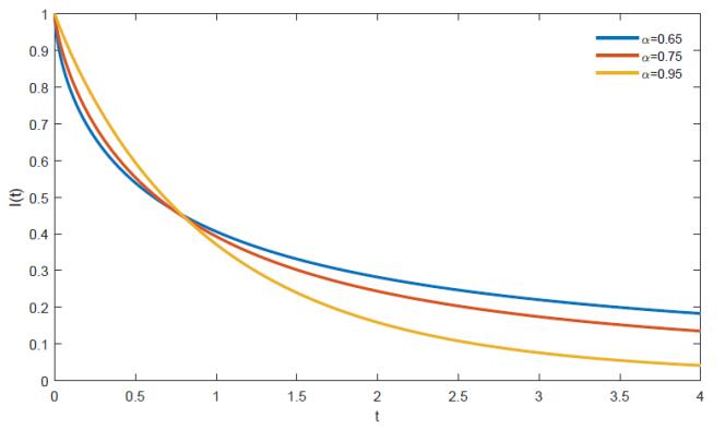
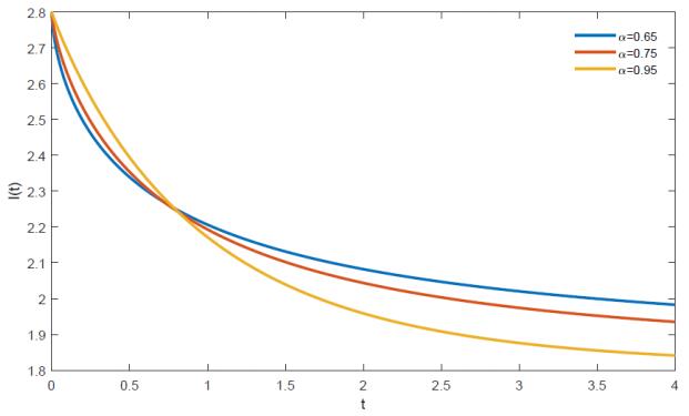
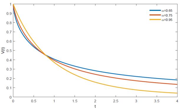
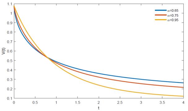
Figures(4)

Ndolane Sene. Fractional input stability for electrical circuits described by the Riemann-Liouville and the Caputo fractional derivatives[J]. AIMS Mathematics, 2019, 4(1): 147-165. doi: 10.3934/Math.2019.1.147


 DownLoad: