Comparative evaluation of nutritional composition, phytochemicals and sensorial attributes of lyophilized vs conventionally dried <i>Grewia asiatica</i> fruit pulp powder

Saima Latif; Muhammad Sohaib; Sanaullah Iqbal; Muhammad Hassan Mushtaq; Muhammad Tauseef Sultan; Saima Latif; Muhammad Sohaib; Sanaullah Iqbal; Muhammad Hassan Mushtaq; Muhammad Tauseef Sultan

doi:10.3934/agrfood.2025013

AIMS Agriculture and Food

2025, Volume 10, Issue 1: 247-265. doi: 10.3934/agrfood.2025013

Previous Article Next Article

Research article

Comparative evaluation of nutritional composition, phytochemicals and sensorial attributes of lyophilized vs conventionally dried Grewia asiatica fruit pulp powder

1.
Department of Food Science & Human Nutrition, University of Veterinary & Animal Science, Syed Abdul Qadir Jilani Outfall Road, Lahore, 54000, Punjab, Pakistan
2.
Department of Epidemiology & Public Health, University of Veterinary and Animal Sciences, Syed Abdul Qadir Jilani Outfall Road, Lahore, 54000, Punjab, Pakistan
3.
Department of Human Nutrition, Bahauddin Zakariya University Multan, Multan, Punjab, Pakistan

Received: 26 August 2024 Revised: 22 February 2025 Accepted: 28 March 2025 Published: 07 April 2025

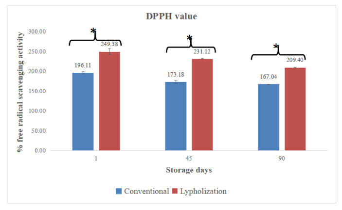
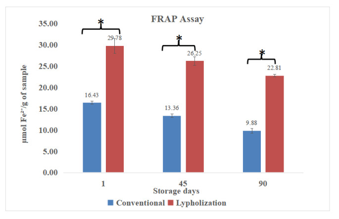
Grewia asiatica, commonly known as phalsa, is a widely cultivated fruit in Pakistan, valued for its nutritional and medicinal benefits. Being a perishable fruit with limited shelf life and rapid spoilage, a preservation approach is needed to extend fruit shelf life and product development. In this context, we aimed to extend the shelf life of G. asiatica fruit pulp using conventional and lyophilization drying and to evaluate their impact on nutritional composition, phytochemicals attributes, sensory evaluation and product shelf life for fruit pulp powder stored at ambient conditions for 3 months (0, 45^th and 90^th day). For the study, ripe G. asiatica fruit sourced from local farms were subjected to cleaning followed by drying using conventional and lyophilization processes. The resulting fruit powder was packed in sealed foil bags and stored at room temperature for 3 months, subjected to nutritional properties, phytochemicals, antioxidant capacity, and sensory evaluation on the 0, 45^th, and 90^th storage days. The results showed that both techniques increased the shelf life of powder. However, lyophilization resulted in better retention of vitamin C, antioxidant activity, and better free radical scavenging activity in fruit powder than conventional drying. Color parameters and sensory evaluation were also affected by drying and storage conditions as an advancement of storage resulted in decreased consumer acceptability. These findings demonstrate that lyophilization effectively preserves nutritional and phytochemical qualities of G. asiatica powder, making it a viable preservation approach for prolonging fruit shelf life while maintaining its health promoting compounds and functional properties. The lyophilized G. asiatica fruit pulp powder may have potential use in the food industry as an additive in ready-to-use products to enhance nutritional attributes, color, and better consumer acceptability for dried powders.

Keywords:

Citation: Saima Latif, Muhammad Sohaib, Sanaullah Iqbal, Muhammad Hassan Mushtaq, Muhammad Tauseef Sultan. Comparative evaluation of nutritional composition, phytochemicals and sensorial attributes of lyophilized vs conventionally dried Grewia asiatica fruit pulp powder[J]. AIMS Agriculture and Food, 2025, 10(1): 247-265. doi: 10.3934/agrfood.2025013

Related Papers:

[1]	M. Mossa Al-Sawalha, Safyan Mukhtar, Azzh Saad Alshehry, Mohammad Alqudah, Musaad S. Aldhabani . Chaotic perturbations of solitons in complex conformable Maccari system. AIMS Mathematics, 2025, 10(3): 6664-6693. doi: 10.3934/math.2025305
[2]	M. B. Almatrafi, Mahmoud A. E. Abdelrahman . The novel stochastic structure of solitary waves to the stochastic Maccari's system via Wiener process. AIMS Mathematics, 2025, 10(1): 1183-1200. doi: 10.3934/math.2025056
[3]	Naseem Abbas, Amjad Hussain, Mohsen Bakouri, Thoraya N. Alharthi, Ilyas Khan . A study of dynamical features and novel soliton structures of complex-coupled Maccari's system. AIMS Mathematics, 2025, 10(2): 3025-3040. doi: 10.3934/math.2025141
[4]	Mohammad Alqudah, Manoj Singh . Applications of soliton solutions of the two-dimensional nonlinear complex coupled Maccari equations. AIMS Mathematics, 2024, 9(11): 31636-31657. doi: 10.3934/math.20241521
[5]	Mahmoud A. E. Abdelrahman, S. Z. Hassan, R. A. Alomair, D. M. Alsaleh . Fundamental solutions for the conformable time fractional Phi-4 and space-time fractional simplified MCH equations. AIMS Mathematics, 2021, 6(6): 6555-6568. doi: 10.3934/math.2021386
[6]	Hammad Alotaibi . Solitary waves of the generalized Zakharov equations via integration algorithms. AIMS Mathematics, 2024, 9(5): 12650-12677. doi: 10.3934/math.2024619
[7]	E. S. Aly, Mahmoud A. E. Abdelrahman, S. Bourazza, Abdullah Ali H. Ahmadini, Ahmed Hussein Msmali, Nadia A. Askar . New solutions for perturbed chiral nonlinear Schrödinger equation. AIMS Mathematics, 2022, 7(7): 12289-12302. doi: 10.3934/math.2022682
[8]	Jamshad Ahmad, Zulaikha Mustafa, Mehjabeen Anwar, Marouan Kouki, Nehad Ali Shah . Exploring solitonic wave dynamics in the context of nonlinear conformable Kairat-X equation via unified method. AIMS Mathematics, 2025, 10(5): 10898-10916. doi: 10.3934/math.2025495
[9]	Azzh Saad Alshehry, Safyan Mukhtar, Ali M. Mahnashi . Optical fractals and Hump soliton structures in integrable Kuralay-Ⅱ system. AIMS Mathematics, 2024, 9(10): 28058-28078. doi: 10.3934/math.20241361
[10]	Yousef F. Alharbi, E. K. El-Shewy, Mahmoud A. E. Abdelrahman . New and effective solitary applications in Schrödinger equation via Brownian motion process with physical coefficients of fiber optics. AIMS Mathematics, 2023, 8(2): 4126-4140. doi: 10.3934/math.2023205

Abstract

1. Introduction

Nonlinear evolution equations (NLEEs) are utilized in order to display many complex phenomena arising in various fields of applied sciences, such as superfluid, chemical engineering, thermal engineering, plasma physics, optical fibers and so on ^{[1,2,3,4,5,6,7,8]}. There are many scientists in various fields of natural sciences are interested in investigation of the nonlinear phenomena. Various vital analytical methods have been proposed and developed to extract the solutions of different kinds of NLEEs, see ^{[9,10,11,12,13,14,15,16,17,18]}. Moreover, there are recent development in studying the dynamics of soliton solutions and analytical closed-form solutions ^{[19,20,21,22,23,24,25,26,27,28,29,30]}.

The Maccari (MS) system, derived by Maccari in 1996 with a reduction technique based on spatio-temporal rescaling, from the Kadomtsev-Petviashvili equation ^[31]. This system is a kind of NLEEs that are often introduced to prescribe the motion of the isolated waves, localized in a small part of space, in various fields such as plasma physics, quantum mechanics, Bose-Einstein condensates, optical fiber communications and so on ^{[32,33,34,35,36,37,38,39]}. Recently, some investigations presented new novel concepts in wave motions and pulses in the study of nonlinear unforeseen critical behaviors such as the electrostatic noise in auroura, the acoustics wave in fluid and telltales wiggle electric fields ^{[40,41,42,43]}.

In this article, we consider the coupled MS ^[32,35,44], given as follows:

$\begin{equation} \begin{array}{l} iQ_t+Q_{xx}+RQ = 0, \\ R_{t}+R_{y}+(\mid Q \mid^2)_{x} = 0, \end{array} \end{equation}$

(1.1)

where $Q = Q(x, y, t)$ denotes the complex scalar field and $R = R(x, y, t)$ denotes the real scalar field. The independent variables are $x, y$ and $t$ denotes the temporal variable.

Also, we can consider the coupled nonlinear MS ^[45], given as follows:

$\begin{equation} \begin{array}{l} iQ_t+Q_{xx}+RQ = 0, \\ i\, S_{t}+S_{xx}+RS = 0, \\ R_{t}+R_{y}+(\mid Q+S \mid^2)_{x} = 0, \end{array} \end{equation}$

(1.2)

where $Q = Q(x, y, t)$ and $S = S(x, y, t)$ denote the complex scalar fields and $R = R(x, y, t)$ denotes the real scalar field.

Moreover, we consider the coupled nonlinear MS ^[34], described as follows:

$\begin{equation} \begin{array}{l} i\, Q_t+Q_{xx}+RQ = 0, \\ i\, S_{t}+S_{xx}+RS = 0, \\ i\, N_{t}+N_{xx}+RN = 0, \\ R_{t}+R_{y}+(\mid Q+S+N \mid^2)_{x} = 0, \end{array} \end{equation}$

(1.3)

where $Q = Q(x, y, t)$ , $S = S(x, y, t)$ , $N = N(x, y, t)$ denote the complex scalar fields and $R = R(x, y, t)$ denotes the real scalar field.

Our study is motivated to grasp some new solutions for the three coupled models of MS by using the unified solver method. This solver introduces some families of solutions in explicit way with free physical parameters. These solutions admit pivotal applications in plasma environments, superfluid, plasma physics, nonlinear optic^[46,47]. The proposed solver will be utilized as a box solver for solving many other nonlinear models arising in applied science and new physics. In contrast to other methods, this solver preserves several advantages, such as, it avoids complex and tedious calculations and presents pivotal solutions in an explicit way. Moreover, this solver is simple, robust, well ordered and efficacious. The proposed solver will be significant for mathematicians, engineers and physicists. To the best of our knowledge, no previous work has been done using the proposed solver for solving the MS systems.

The present article is organized as follows. Section 2 describes the unified solver technique. Section 3 presents the solutions for three coupled of the Maccari's systems. Section 4 gives the physical interpretation of the presented results. Moreover, some graphs of some acquired solutions are depicted. Conclusions and future directions for research are all reported in Section 5.

2. Unified solver method

We give the unified solver for the widely used NLEEs arising in the nonlinear science. For a given NLEE with some physical field $\Psi(x, y, t)$

$\begin{equation} F(\Psi , \Psi _{t}, \Psi _{x}, \Psi _{tt}, \Psi _{xx}, ....) = 0, \end{equation}$

(2.1)

we construct its explicit solutions in the form:

$\begin{equation} \Psi (x, y, t) = \Psi (\xi ), \ \xi = k_1 x+k_2 y+k_3t, \end{equation}$

(2.2)

where $k_1$ , $k_2$ and $k_3$ are constants. Consequently the nonlinear evolution Eq (2.1) transformed to the following ordinary differential equation (ODE):

$\begin{equation} G(\Psi , \Psi ^{\prime }, \Psi ^{\prime \prime }, \Psi ^{\prime \prime \prime}, ...) = 0. \end{equation}$

(2.3)

Based on He's semi-inverse method ^[48,49,50], if possible, integrate (2.3) term by term one or more times. The variational model for the differential Eq (2.3) can be obtained by the semi-inverse method ^[51] which reads:

$\begin{equation} J(\Psi) = \underset{0}{\overset{\infty}{\int}}L\, d\xi, \end{equation}$

(2.4)

where $L$ is the Lagrangian function, of the problem described by the Eq (2.3), depending on $\Psi$ and its derivatives given in the form:

$\begin{equation} L = \frac{1}{2}\Psi^{^{\prime}2}-V, \end{equation}$

(2.5)

where $V$ is the potential function. By a Ritz method, we can find different forms of solitary wave solutions, such as $\Psi(x, y, t) = \alpha$ $\mbox{sech}(\beta \xi)$ , $\Psi(x, y, t) = \alpha$ $\mbox{csch}(\beta \xi)$ , $\Psi(x, y, t) = \alpha$ $\mbox{tanh}(\beta \xi)$ , $\Psi(x, y, t) = \alpha$ $\mbox{cotch}(\beta \xi)$ and $\Psi(x, y, t) = \alpha$ $\mbox{sech}^2(\beta \xi)$ where $\alpha$ and $\beta$ are constants determined later.

We look for a solitary wave solution in the form

$\begin{equation} \Psi(x, y, t) = \alpha, \mbox{sech}(\beta \xi), \Psi(x, y, t) = \alpha, \mbox{sech}^2(\beta \xi), \Psi(x, y, t) = \alpha, \tanh(\beta \xi). \end{equation}$

(2.6)

In this section we give the unified solver for the widely used NLEEs arising in the nonlinear science. Suppose a system of equations can be reduced to the form:

$\begin{equation} L_{1}\Psi^{\prime\prime}+L_{2}\Psi^{3}+L_{3}\Psi = 0, \end{equation}$

(2.7)

where $L_{i}, i = 1, 2, 3$ are constants. Multiplying (2.7) by $\Psi^{^{\prime}}$ and integrating with respect to $\Psi$ we get the equation:

$\begin{equation} \frac{1}{2}\Psi^{^{\prime}2}+\frac{L_2}{4L_1} \Psi^{4}+\frac{L_3}{2L_1} \Psi^{2}+L_{0} = 0 \end{equation}$

(2.8)

and $L_{0}$ is a constant of integration. Thus the Eq (2.7) can be written in the form:

$\begin{equation} \Psi^{\prime\prime} = -\frac{\partial V}{\partial\Psi}, \; V = -(\gamma_{2}\Psi ^{4}+\gamma_{1}\psi^{2}+\gamma _{0}), \end{equation}$

(2.9)

where

$\begin{equation} \gamma_2 = -\frac{L_2}{4L_1}, \gamma_1 = -\frac{L_3}{2L_1}, \gamma_{0} = - L_0 \end{equation}$

(2.10)

and $V$ is the potential function (Sagadev potential).

We apply He's semi-inverse technique^[48,49,50] for solving Eq (2.7), which construct the following variational formulation from Eq (2.8)

$\begin{equation} J = \int_{0}^{\infty}\left[\frac{1}{2}\Psi^{\prime2}+\gamma_{2}\Psi^{4}+\gamma_{1}\Psi^{2}+\gamma_{0}\right] d\xi. \end{equation}$

(2.11)

By Ritz-like method, we look for a solitary wave solution in the form given by Eq (2.6). Substituting from Eq (2.6) into Eq (2.11) and making $J$ stationary with respect to $\alpha$ and $\beta$ we obtain:

$\begin{equation} \frac{\partial J}{\partial \alpha} = 0;\; \frac{\partial J}{\partial \beta} = 0. \end{equation}$

(2.12)

Solving simultaneously the system of equations given by (2.12) we obtain $\alpha$ and $\beta$ . Consequently the solitary wave solution given by Eq (2.6) is well determined.

2.1. The first family

The first family of solutions takes the form:

$\begin{equation} \Psi(\xi) = \alpha\, \mbox{sech}^{{}}\theta, \; \theta = \beta\xi. \end{equation}$

(2.13)

Substituting from Eq (2.13) in Eq (2.11), we get

$\begin{align*} J & = \frac{1}{\beta}\int_{0}^{\infty}[\frac{1}{2}\alpha^{2}\beta^{2}, \mbox{sech}^{2}, \theta\; \mbox{tanh}^{2}\theta+ \gamma_2, \alpha^{4} \mbox{sech}^{4}\theta+\gamma_1 , \alpha^{2}\mbox{sech}^{2}\theta+\gamma_{0}]d\theta. \end{align*}$

Since $\gamma_{0}$ is a constant of integration we can let $\gamma_{0} = 0$ and consequently:

$\begin{align} J = \frac{\alpha}{12 \beta}\left[ 2\alpha \beta^{2}+8\gamma_{2}\alpha^{3}+12 \gamma_{1}\alpha\right]. \end{align}$

(2.14)

Making $J$ stationary with respect to $\alpha$ and $\beta$ leads to

$\begin{equation} \frac{\partial J}{\partial \alpha} = \frac{1}{12\beta}\left[ 32\gamma_{2}\alpha^{3}+24\gamma_{1}\alpha+4\alpha\beta^2\right] = 0, \end{equation}$

(2.15)

$\begin{equation} \frac{\partial J}{\partial \beta} = -\frac{\alpha}{12\beta^{2}}\left[ 8\gamma_{2}\alpha^{3}+12\gamma_{1}\alpha-2\alpha\beta^{2}\right] = 0. \end{equation}$

(2.16)

Solving these equations and using (2.13), the solutions of Eq (2.9) take the form:

$\begin{equation} \Psi(\xi) = \pm\sqrt{\frac{-\gamma_1}{\gamma_2}}, \mbox{sech}\left(\pm\sqrt{2\gamma_{1}}\xi\right). \end{equation}$

(2.17)

Consequently by using (2.10) the first family of solutions takes the form:

$\begin{equation} \Psi(\xi) = \pm \sqrt{\frac{-2L_3}{L_2}}, \mbox{sech}\left( \pm \sqrt{-\frac{L_3}{L_1}}\xi\right). \end{equation}$

(2.18)

2.2. The second family

The second family of solutions takes the form:

$\begin{equation} \psi(\xi) = \alpha\, \mbox{sech}^{2}\theta\; ;\theta = \beta\xi. \end{equation}$

(2.19)

The substitution from Eq (2.19) in Eq (2.11) leads to

$\begin{align*} J & = \frac{\alpha}{\beta}\int_{0}^{\infty}[2\alpha \beta^{2}\mbox{sech}^{4}\theta\; \mbox{tanh}^{2}\theta+\gamma_{2}\alpha^{3} \mbox{sech}^{8}\theta+ \gamma_{1} \alpha\, \mbox{sech}^{4}\theta+\frac{\gamma_{0}}{\alpha}] d\theta. \end{align*}$

Assuming that $\gamma_{0} = 0$ we find that

$\begin{equation} J = \frac{2\alpha^{2}}{105\beta}\left[ 14\alpha \beta^{2}+24\gamma_{2}\alpha^{3}+35 \gamma_{1}\alpha\right]. \end{equation}$

(2.20)

Making $J$ stationary with respect to $\alpha$ and $\beta$ leads to

$\begin{align} 14\alpha \beta^{2}+48\gamma_{2}\alpha^{3}+35\gamma_{1}\alpha & = 0, \end{align}$

(2.21)

$\begin{align} 14\alpha \beta^{2}-24\gamma_{2} \alpha^{3}-35\gamma_{1}\alpha & = 0. \end{align}$

(2.22)

Solving these equations and using (2.19), the second family of solutions of Eqs (2.9) and (2.7) take the form:

$\begin{equation} \Psi(\xi) = \pm \sqrt{\frac{-35\gamma_{1}}{36\gamma_{2}}}\, \mbox{sech}^{2}\left( \pm \sqrt{\frac{5}{6}\gamma_{1}} \, \xi\right) \end{equation}$

(2.23)

and

$\begin{equation} \Psi(\xi) = \pm\sqrt{\frac{-35\, L_{3}}{18\, L_{2}}} \mbox{sech}^{2}\left( \pm \sqrt{-\frac{5\, L_{3}}{12\, L_{1}}} \, \xi\right), \end{equation}$

(2.24)

respectively.

2.3. The third family

The third family of solutions takes the form:

$\begin{equation} \psi (\xi ) = \alpha, \tanh (\beta\xi ). \end{equation}$

(2.25)

Substituting from Eq (2.25) into Eq (2.11), we have

$\begin{align*} J & = \frac{1}{\beta}\int_{0}^{\infty}[\frac{1}{2}\alpha^{2}\, \beta^{2}\, \mbox{sech}^{4}\theta +\gamma_{2}\alpha^{4}\tanh^{4}\theta+ \gamma_{1}\, \alpha^{2}\tanh^{2}\theta+ \gamma_{0}]d\theta \\ & = \frac{1}{\beta}\int_{0}^{\infty}[\alpha^{2}( \gamma_{2}\alpha^{2}+\frac{1}{2} \beta^{2})\, \mbox{sech}^{4}\theta-\alpha^{2}(2 \gamma_{2} \alpha^{2}+\gamma_{1})\, \mbox{sech}^{2}\theta ]d\theta \\& +\frac{1}{\beta}(\gamma_{2}\alpha^{4}+ \gamma_{1}\alpha^{2}+\gamma_{0})\int_{0}^{\infty }d\theta \notag. \end{align*}$

Under the condition

$\begin{equation} \gamma_{0} = -\alpha^{2}(\gamma_{2} \alpha^{2}+\gamma_{1}), \end{equation}$

(2.26)

we find that

$\begin{align} J & = \frac{-\alpha^{2}}{3\beta}\left[ 4\gamma_{2}\alpha^{2}+3\gamma _{1}-\beta^{2}\right]. \end{align}$

(2.27)

The values of $\alpha$ and $\beta$ which makes $J$ stationary with respect to $\alpha$ and $\beta$ are obtained by solving the two conditions

$\begin{align} \frac{\partial J}{\partial \alpha} & = \frac{-\alpha}{3\beta}\left[ 16\gamma_{2}\alpha^{2}+6\gamma_{1}-2\beta^{2}\right] = 0, \end{align}$

(2.28)

$\begin{align} \frac{\partial J}{\partial \beta} & = \frac{\alpha^{2}}{3\beta^{2}}\left[ 4\gamma_{2}\alpha^{2}+3\gamma_{1}+\beta^{2}\right] = 0. \end{align}$

(2.29)

Solving these equations and using (2.25), the solutions of Eq (2.9) take the form:

$\begin{equation} \Psi(\xi) = \pm\sqrt{\frac{-\gamma_{1}}{2\, \gamma_{2}}} \tanh\left( \pm \sqrt{-\gamma_{1}}\xi\right). \end{equation}$

(2.30)

Consequently the third family of solutions of (2.7) take the form:

$\begin{equation} \Psi(\xi) = \pm\sqrt{\frac{-L_{3}}{L_{2}}} \tanh\left( \pm \sqrt{\frac{L_3}{2L_1}}\xi\right). \end{equation}$

(2.31)

3. Applications

In this section we introduce the solutions for the coupled nonlinear Maccari's systems.

3.1. Solutions of system (1.1)

Utilizing the wave transformation:

$\begin{equation} \begin{split} Q(x, y, t) = &e^{i(kx+\alpha\, y+\lambda\, t)}u(\zeta), \; \; \; R(x, y, t) = R(\zeta), \zeta = x + \beta y -2k t, \end{split} \end{equation}$

(3.1)

$k, \alpha, \lambda$ and $\beta$ are constants. Then the system of Eq (1.1) is converted to the following system

$\begin{equation} \begin{array}{l} u''+u R-(\lambda+k^2)u = 0, \\ (u^2)'-(2k-\beta)R' = 0. \end{array} \end{equation}$

(3.2)

Integrating second equation of Eq (3.2) and taking integration constant as zero, gives

$\begin{equation} R = \left(\frac{1}{2k-\beta}\right)u^2. \end{equation}$

(3.3)

Substituting Eq (3.3) into first equation of system (3.2), yields

$\begin{equation} L_{1} u''+L_{2}u^3+L_{3}u = 0, \end{equation}$

(3.4)

where

$\begin{equation} L_{1} = 1, L_{2} = \frac{1}{2k-\beta}, L_{3} = -(\lambda+k^2). \end{equation}$

(3.5)

Applying the unified solver method described in Section 2, three families of solutions of Eq (1.1) are given as follows:

3.1.1. The first family of solutions

$\begin{equation} u_{1, 2}(\zeta) = \pm \sqrt{2 (2k-\beta)(\lambda+k^2)}\, \mbox{sech}\left( \pm \sqrt{\lambda+k^2}\, \zeta\right). \end{equation}$

(3.6)

Thus,

$\begin{equation} Q_{1, 2}(x, y, t) = \pm e^{i(kx+\alpha\, y+\lambda\, t)}\sqrt{2 (2k-\beta)(\lambda+k^2)}\, \mbox{sech}\left( \pm \sqrt{\lambda+k^2}\, \zeta\right). \end{equation}$

(3.7)

$\begin{equation} R_{1, 2}(x, y, t) = 2(\lambda+k^2)\, \mbox{sech}^{2}\left( \pm \sqrt{\lambda+k^2}\, \zeta\right), \; \; \; \lambda+k^2 > 0. \end{equation}$

(3.8)

3.1.2. The second family of solutions

$\begin{equation} u_{3, 4}(\zeta) = \pm \sqrt{\frac{35(\lambda+k^2)(2k-\beta)}{18}}\, \mbox{sech}^{2}\left( \pm \sqrt{\frac{5(\lambda+k^2)}{12}} \, \zeta\right). \end{equation}$

(3.9)

Thus,

$\begin{equation} Q_{3, 4}(x, y, t) = \pm e^{i(kx+\alpha\, y+\lambda\, t)} \sqrt{\frac{35(\lambda+k^2)(2k-\beta)}{18}}\, \mbox{sech}^{2}\left( \pm \sqrt{\frac{5(\lambda+k^2)}{12}} \, \zeta\right). \end{equation}$

(3.10)

$\begin{equation} R_{3, 4}(x, y, t) = \frac{35(\lambda+k^2)}{18}\, \mbox{sech}^{4}\left( \pm\sqrt{ \frac{5(\lambda+k^2)}{12}} \, \zeta\right) , \; \; \; \lambda+k^2 > 0. \end{equation}$

(3.11)

3.1.3. The third family of solutions

$\begin{equation} u_{5, 6}(\zeta) = \pm\sqrt{(\lambda+k^2)(2k-\beta)} \tanh\left( \pm \sqrt{-\frac{(\lambda+k^2)}{2}}\zeta\right). \end{equation}$

(3.12)

Thus,

$\begin{equation} Q_{5, 6}(x, y, t) = \pm\, e^{i(k+\alpha\, y+\lambda\, t)}\sqrt{(\lambda+k^2)(2k-\beta)} \tanh\left( \pm \sqrt{-\frac{\lambda+k^2}{2}}\zeta\right). \end{equation}$

(3.13)

$\begin{equation} R_{5, 6}(x, y, t) = (\lambda+k^2) \tanh^{2}\left( \pm \sqrt{-\frac{\lambda+k^2}{2}}\zeta\right), \; \; \lambda+k^2 < 0. \end{equation}$

(3.14)

3.2. Solutions of system (1.2)

Consider the wave transformation:

$\begin{equation} \begin{split} Q(x, y, t)& = e^{i(kx+\alpha\, y+\lambda\, t)}u(\zeta), \\ S(x, y, t)& = e^{i(kx+\alpha\, y+\lambda\, t)}v(\zeta), \\ R(x, y, t)& = R(\xi), \zeta = x + \beta y -2k t, \end{split} \end{equation}$

(3.15)

where $k, \alpha, \lambda$ and $\beta$ are constants. By applying this transformation to the system (1.2) we get

$\begin{equation} \begin{array}{l} u''-(\lambda+k^2) u + u R = 0, \\ v''-(\lambda+k^2) v + v R = 0, \\ ((u+v)^2)'-(2k-\beta)R' = 0. \end{array} \end{equation}$

(3.16)

Integrating third equation of the system of Eq (3.16) and taking integration constant as zero, gives

$\begin{equation} R = \left(\frac{1}{2k-\beta}\right)(u+v)^2. \end{equation}$

(3.17)

Substituting Eq (3.17) into first two equations of (3.16), yields

$\begin{equation} \begin{array}{l} u''+ \frac{1}{2k-\beta}u(u+v)^2-(\lambda+k^2)u = 0, \\ v''+ \frac{1}{2k-\beta}v(u+v)^2-(\lambda+k^2)v = 0. \end{array} \end{equation}$

(3.18)

In order to solve the last system of equations, we use a simple relation between $u$ and $v$ , as follows:

$\begin{equation} v = r\, u, \end{equation}$

(3.19)

where $r$ is an arbitrary constant. Substituting (3.19) into the system (3.18), gives

$\begin{equation} \Gamma_{1} u''+\Gamma_{2}u^3+\Gamma_{3}u = 0, \end{equation}$

(3.20)

where $\Gamma_{1} = 1, \Gamma_{2} = \frac{(1+r)^2}{2k-\beta}, \Gamma_{3} = -(\lambda+k^2)$ .

In view of the unified solver illustrated in Section 2 solutions of Eq (1.2) can be given in the following formulas:

3.2.1. The first family of solutions

$\begin{equation} u_{1, 2}(\zeta) = \pm \sqrt{\frac{2(\lambda+k^2)(2k-\beta)}{(1+r)^2}}\, \mbox{sech}\left( \pm \sqrt{\lambda+k^2}\zeta\right). \end{equation}$

(3.21)

Thus,

$\begin{equation} v_{1, 2}(\zeta) = \pm r \sqrt{\frac{2(\lambda+k^2)(2k-\beta)}{(1+r)^2}}\, \mbox{sech}\left( \pm \sqrt{\lambda+k^2}\zeta\right). \end{equation}$

(3.22)

$\begin{equation} Q_{1, 2}(x, y, t) = \pm e^{i(kx+\alpha\, y+\lambda\, t)}\sqrt{\frac{2(\lambda+k^2)(2k-\beta)}{(1+r)^2}}\, \mbox{sech}\left( \pm \sqrt{\lambda+k^2}\zeta\right). \end{equation}$

(3.23)

$\begin{equation} S_{1, 2}(x, y, t) = \pm r e^{i(kx+\alpha\, y+\lambda\, t)}\sqrt{\frac{2(\lambda+k^2)(\beta-2k)}{(1+r)^2}}\, \mbox{sech}\left( \pm \sqrt{\lambda+k^2}\zeta\right). \end{equation}$

(3.24)

$\begin{equation} R_{1, 2}(x, y, t) = 2(\lambda+k^2)\mbox{sech}^2\left( \pm \sqrt{\lambda+k^2}\xi\right), \lambda+k^2 > 0. \end{equation}$

(3.25)

3.2.2. The second family of solutions

$\begin{equation} u_{3, 4}(\zeta) = \pm \sqrt{\frac{35(\lambda+k^2)(2k-\beta)}{18(1+r)^2}}\, \mbox{sech}^2\left( \pm \sqrt{\frac{5}{12}(\lambda+k^2)}\zeta\right). \end{equation}$

(3.26)

Thus,

$\begin{equation} v_{3, 4}(\zeta) = \pm r \sqrt{\frac{35(\lambda+k^2)(2k-\beta)}{18(1+r)^2}}\, \mbox{sech}^2\left( \pm \sqrt{\frac{5}{12}(\lambda+k^2)}\zeta\right). \end{equation}$

(3.27)

$\begin{equation} Q_{3, 4}(x, y, t) = \pm e^{i(kx+\alpha\, y+\lambda\, t)}\sqrt{\frac{35(\lambda+k^2)(2k-\beta)}{18(1+r)^2}}\, \mbox{sech}^2\left( \pm \sqrt{\frac{5}{12}(\lambda+k^2)}\zeta\right). \end{equation}$

(3.28)

$\begin{equation} S_{3, 4}(x, y, t) = \pm r e^{i(kx+\alpha\, y+\lambda\, t)}\sqrt{\frac{35(\lambda+k^2)(2k-\beta)}{18(1+r)^2}}\, \mbox{sech}^2\left( \pm \sqrt{\frac{5}{12}(\lambda+k^2)}\zeta\right). \end{equation}$

(3.29)

$\begin{equation} R_{3, 4}(x, y, t) = \frac{35}{18}(\lambda+k^2)\mbox{sech}^4\left( \pm \sqrt{\frac{5}{12}(\lambda+k^2)}\xi\right), \; \; \lambda+k^2 > 0. \end{equation}$

(3.30)

3.2.3. The third family of solutions

$\begin{equation} u_{5, 6}(\zeta) = \pm \sqrt{\frac{(\lambda+k^2)(2k-\beta)}{(1+r)^2}}\, \tanh\left( \pm \sqrt{-\frac{\lambda+k^2}{2}}\zeta\right). \end{equation}$

(3.31)

Thus,

$\begin{equation} v_{5, 6}(\zeta) = \pm r\sqrt{\frac{(\lambda+k^2)(2k-\beta)}{(1+r)^2}}\, \tanh\left( \pm \sqrt{-\frac{\lambda+k^2}{2}}\zeta\right). \end{equation}$

(3.32)

$\begin{equation} Q_{5, 6}(x, y, t) = \pm e^{i(kx+\alpha\, y+\lambda\, t)} \sqrt{\frac{(\lambda+k^2)(2k-\beta)}{(1+r)^2}}\, \tanh\left( \pm \sqrt{-\frac{\lambda+k^2}{2}}\zeta\right). \end{equation}$

(3.33)

$\begin{equation} S_{5, 6}(x, y, t) = \pm re^{i(kx+\alpha\, y+\lambda\, t)} \sqrt{\frac{(\lambda+k^2)(2k-\beta)}{(1+r)^2}}\, \tanh\left( \pm \sqrt{-\frac{\lambda+k^2}{2}}\zeta\right). \end{equation}$

(3.34)

$\begin{equation} R_{5, 6}(x, y, t) = (\lambda+k^2)\tanh^2\left( \pm \sqrt{-\frac{\lambda+k^2}{2}}\zeta\right), \; \; \lambda+k^2 < 0. \end{equation}$

(3.35)

3.3. Solutions of system (1.3)

In order to solve the system of Eq (1.3), we first consider the following wave transformation:

$\begin{equation} \begin{split} Q(x, y, t)& = e^{i(kx+\alpha\, y+\lambda\, t)}u(\zeta), \\ S(x, y, t)& = e^{i(kx+\alpha\, y+\lambda\, t)}v(\zeta), \\ N(x, y, t)& = e^{i(kx+\alpha\, y+\lambda\, t)}w(\zeta), \\ R(x, y, t)& = R(\zeta), \; \zeta = x + \beta y -2k t, \end{split} \end{equation}$

(3.36)

where $k, \alpha, \lambda$ and $\beta$ are constants. Substituting this transformation to system (1.3) gives

$\begin{equation} \begin{array}{l} u''-(\lambda+k^2) u + u R = 0, \\ v''-(\lambda+k^2) v + v R = 0, \\ w''-(\lambda+k^2) w + w R = 0, \\ ((u+v+w)^2)' -(2k-\beta)R' = 0. \end{array} \end{equation}$

(3.37)

As illustrated before, we integrate the third equation of (3.37) with assuming the integration constant to be zero and this gives

$\begin{equation} R = \left(\frac{1}{2k-\beta}\right)(u+v+w)^2. \end{equation}$

(3.38)

Substituting Eq (3.38) into first three equation of (3.37), implies

$\begin{equation} \begin{array}{l} u''+ \frac{1}{2k-\beta}u(u+v+w)^2-(\lambda+k^2)u = 0, \\ v''+ \frac{1}{2k-\beta}v(u+v)^2-(\lambda+k^2)v = 0, \\ w''+ \frac{1}{2k-\beta}w(u+v+w)^2-(\lambda+k^2)w = 0. \end{array} \end{equation}$

(3.39)

To solve these equations, we use a simple relations between $v, w$ and $u$ , as follows

$\begin{equation} v = r_{1}\, u, \; \; \; w = r_{2}\, u, \end{equation}$

(3.40)

where $r_{1}, r_{2}$ are arbitrary constants. Substituting (3.40) into the Eq (3.39), gives

$\begin{equation} \Gamma_{1} u''+\Gamma_{2}u^3+\Gamma_{3}u = 0, \end{equation}$

(3.41)

where $\Gamma_{1} = 1, \Gamma_{2} = \frac{(1+r_{1}+r_{2})^2}{2k-\beta}, \Gamma_{3} = -(\lambda+k^2)$ .

Similarly, solutions of system (1.3) can be obtained using the unified solver, presented in Section 2, and are described in the following:

3.3.1. The first family of solutions

$\begin{equation} u_{1, 2}(\zeta) = \pm \sqrt{\frac{2(\lambda+k^2)(2k-\beta)}{(1+r_1+r_2)^2}}\, \mbox{sech}\left( \pm \sqrt{\lambda+k^2}\zeta\right). \end{equation}$

(3.42)

Thus,

$\begin{equation} v_{1, 2}(\zeta) = \pm r_1 \sqrt{\frac{2(\lambda+k^2)(2k-\beta)}{(1+r_1+r_2)^2}}\, \mbox{sech}\left( \pm \sqrt{\lambda+k^2}\zeta\right). \end{equation}$

(3.43)

$\begin{equation} w_{1, 2}(\zeta) = \pm r_2 \sqrt{\frac{2(\lambda+k^2)(2k-\beta)}{(1+r_1+r_2)^2}}\, \mbox{sech}\left( \pm \sqrt{\lambda+k^2}\zeta\right). \end{equation}$

(3.44)

$\begin{equation} Q_{1, 2}(x, y, t) = \pm e^{i(kx+\alpha\, y+\lambda\, t)}\sqrt{\frac{2(\lambda+k^2)(2k-\beta)}{(1+r_1+r_2)^2}}\, \mbox{sech}\left( \pm \sqrt{\lambda+k^2}\zeta\right). \end{equation}$

(3.45)

$\begin{equation} S_{1, 2}(x, y, t) = \pm r_1 e^{i(kx+\alpha\, y+\lambda\, t)}\sqrt{\frac{2(\lambda+k^2)(2k-\beta)}{(1+r_1+r_2)^2}}\, \mbox{sech}\left( \pm \sqrt{\lambda+k^2}\zeta\right). \end{equation}$

(3.46)

$\begin{equation} N_{1, 2}(x, y, t) = \pm r_2 e^{i(kx+\alpha\, y+\lambda\, t)}\sqrt{\frac{2(\lambda+k^2)(2k-\beta)}{(1+r_1+r_2)^2}}\, \mbox{sech}\left( \pm \sqrt{\lambda+k^2}\zeta\right). \end{equation}$

(3.47)

$\begin{equation} R_{1, 2}(x, y, t) = 2(\lambda+k^2)\, \mbox{sech}^2\left( \pm \sqrt{\lambda+k^2}\zeta\right), \; \; \lambda+k^2 > 0. \end{equation}$

(3.48)

3.3.2. The second family of solutions

$\begin{equation} u_{3, 4}(\zeta) = \pm \sqrt{\frac{35(\lambda+k^2)(2k-\beta)}{18(1+r_1+r_2)^2}}\, \mbox{sech}^2\left( \pm \sqrt{\frac{5}{12}(\lambda+k^2)}\zeta\right). \end{equation}$

(3.49)

Thus,

$\begin{equation} v_{3, 4}(\zeta) = \pm r_1 \sqrt{\frac{35(\lambda+k^2)(2k-\beta)}{18(1+r_1+r_2)^2}}\, \mbox{sech}^2\left( \pm \sqrt{\frac{5}{12}(\lambda+k^2)}\zeta\right). \end{equation}$

(3.50)

$\begin{equation} w_{3, 4}(\zeta) = \pm r_2 \sqrt{\frac{35(\lambda+k^2)(2k-\beta)}{18(1+r_1+r_2)^2}}\, \mbox{sech}^2\left( \pm \sqrt{\frac{5}{12}(\lambda+k^2)}\zeta\right). \end{equation}$

(3.51)

$\begin{equation} Q_{3, 4}(x, y, t) = \pm e^{i(kx+\alpha\, y+\lambda\, t)}\sqrt{\frac{35(\lambda+k^2)(2k-\beta)}{18(1+r_1+r_2)^2}}\, \mbox{sech}^2\left( \pm \sqrt{\frac{5}{12}(\lambda+k^2)}\zeta\right). \end{equation}$

(3.52)

$\begin{equation} S_{3, 4}(x, y, t) = \pm r_1 e^{i(kx+\alpha\, y+\lambda\, t)}\sqrt{\frac{35(\lambda+k^2)(2k-\beta)}{18(1+r_1+r_2)^2}}\, \mbox{sech}^2\left( \pm \sqrt{\frac{5}{12}(\lambda+k^2)}\zeta\right). \end{equation}$

(3.53)

$\begin{equation} N_{3, 4}(x, y, t) = \pm r_2 e^{i(kx+\alpha\, y+\lambda\, t)}\sqrt{\frac{35(\lambda+k^2)(2k-\beta)}{18(1+r_1+r_2)^2}}\, \mbox{sech}^2\left( \pm \sqrt{\frac{5}{12}(\lambda+k^2)}\zeta\right). \end{equation}$

(3.54)

$\begin{equation} R_{3, 4}(x, y, t) = \frac{35}{18}(\lambda+k^2)\mbox{sech}^4\left(\pm \sqrt{\frac{5}{12}(\lambda+k^2)}\zeta\right), \; \; \lambda+k^2 > 0. \end{equation}$

(3.55)

3.3.3. The third family of solutions

$\begin{equation} u_{5, 6}(\zeta) = \pm \sqrt{\frac{(\lambda+k^2)(2k-\beta)}{(1+r_1+r_2)^2}}\, \tanh\left( \pm \sqrt{-\frac{\lambda+k^2}{2}}\zeta\right). \end{equation}$

(3.56)

Thus,

$\begin{equation} v_{5, 6}(\zeta) = \pm r_1 \sqrt{\frac{(\lambda+k^2)(2k-\beta)}{(1+r_1+r_2)^2}}\, \tanh\left( \pm \sqrt{-\frac{\lambda+k^2}{2}}\zeta\right). \end{equation}$

(3.57)

$\begin{equation} w_{5, 6}(\zeta) = \pm r_2 \sqrt{\frac{(\lambda+k^2)(2k-\beta)}{(1+r_1+r_2)^2}}\, \tanh\left( \pm \sqrt{ -\frac{\lambda+k^2}{2}}\zeta\right). \end{equation}$

(3.58)

$\begin{equation} Q_{5, 6}(x, y, t) = \pm\, e^{i(kx+\alpha\, y+\lambda\, t)}\sqrt{\frac{(\lambda+k^2)(2k-\beta)}{(1+r_1+r_2)^2}}\, \tanh\left( \pm \sqrt{-\frac{\lambda+k^2}{2}}\zeta\right). \end{equation}$

(3.59)

$\begin{equation} S_{5, 6}(x, y, t) = \pm r_1 e^{i(kx+\alpha\, y+\lambda\, t)}\sqrt{\frac{(\lambda+k^2)(2k-\beta)}{(1+r_1+r_2)^2}}\, \tanh\left( \pm \sqrt{-\frac{\lambda+k^2}{2}}\zeta\right). \end{equation}$

(3.60)

$\begin{equation} N_{5, 6}(x, y, t) = \pm r_2 e^{i(kx+\alpha\, y+\lambda\, t)}\sqrt{\frac{(\lambda+k^2)(2k-\beta)}{(1+r_1+r_2)^2}}\, \tanh\left( \pm \sqrt{-\frac{\lambda+k^2}{2}}\zeta\right). \end{equation}$

(3.61)

$\begin{equation} R_{5, 6}(x, y, t) = (\lambda+k^2) \tanh^{2}\left( \pm \sqrt{-\frac{\lambda+k^2}{2}}\zeta\right), \; \; \lambda+k^2 < 0. \end{equation}$

(3.62)

4. Results and discussions

Some new solutions for three coupled nonlinear Maccari's systems were achieved in explicit form. These systems are the complex nonlinear models that characteristic the dynamics of isolated waves, confined in a small part of space, in some fields such as plasma physics, superfluid and optical fiber communications ^[35,45]. The acquired solutions are hyperbolic function solutions. These solutions explain some interesting physical phenomena in applied science and new physics. E.g., the hyperbolic secant arises in the profile of a laminar jet whereas the hyperbolic tangent emerges in the study of magnetic moment and special relativity. Indeed, the presented solutions included bright and dark and soliton solutions of the nonlinear Maccari's systems.

According to the presented results in Section 3 we found that

1) The last model generalize the first two models.

2) There is no change in the form of the real field $R(x, y, t)$ in the three models.

Remark 1. 1) The proposed solver in this study can be implemented for the wide classes of nonlinear stochastic partial differential equations (NSPDEs).

2) The proposed solver can be easily extended for solving nonlinear stochastic fractional partial differential equations (NSFPDEs) ^[52,53,54].

3) The proposed solver averts monotonous and complex computations and introduces vital solutions in an explicit form.

For certain values of the parameters in each three cases, Figures 1–6 display the nonlinear dynamical behaviour of the bright and dark soliton solutions.

Figure 1. 3D profile of bright soliton solution for Eq (1.1).

DownLoad: Full-Size Img PowerPoint

Figure 2. 3D profile of dark soliton solution for Eq (1.1).

DownLoad: Full-Size Img PowerPoint

Figure 3. 3D profile of bright soliton solution for Eq (1.2).

DownLoad: Full-Size Img PowerPoint

Figure 4. 3D profile of dark soliton solution for Eq (1.2).

DownLoad: Full-Size Img PowerPoint

Figure 5. 3D profile of bright soliton solution for Eq (1.3).

DownLoad: Full-Size Img PowerPoint

Figure 6. 3D profile of dark soliton solution for Eq (1.3).

DownLoad: Full-Size Img PowerPoint

5. Conclusions

In this article, three coupled nonlinear Maccari's systems were solved using the unified solver technique. Some vital soliton solutions are presented. These solutions have vital physical aspects in many fields such as nonlinear optics plasma physics, hydrodynamic. In the view of such information, it has been seen that the unified solver method has been influential for the analytical solutions of nonlinear Maccari's systems and it is highly effective and reliable in terms of finding new solutions. Moreover, our analysis shows that the proposed solver is simple, powerful and efficient. Some graphs are presented to prescribe the dynamical behaviour of selected solutions. Finally, the used solver can be applied for so many other models emerging in natural science.

Conflict of interest

The authors declare that they have no known competing financial interests or personal relationships that could have appeared to influence the work reported in this paper.

References

[1]	Zia-Ul-Haq M, Stanković MS, Rizwan K, et al. (2015) Compositional study and antioxidant capacity of Grewia asiatica L. seeds grown in Pakistan. Molecules 18: 2663–2676. https://doi.org/10.3390/molecules18032663 doi: 10.3390/molecules18032663
[2]	Khan RS, Asghar W, Khalid N, et al. (2019) Phalsa (Grewia asiatica L) fruit berry a promising functional food ingredient: A comprehensive review. J Berry Res 9: 179–193. https://doi.org/10.3233/JBR-180332 doi: 10.3233/JBR-180332
[3]	Barkaoui S, Madureira J, Mihoubi Boudhrioua N, et al. (2023) Berries: effects on health, preservation methods, and uses in functional foods: A review. Eur Food Res Technol 249: 1–27. https://doi.org/10.1007/s00217-023-04257-2 doi: 10.1007/s00217-023-04257-2
[4]	Ahmad K, Afridi M, Khan N, et al. (2021) Quality deterioration of postharvest fruits and vegetables in developing country Pakistan: A mini overview. Asian J Agric Food Sci 9: 83–90. http://dx.doi.org/10.24203/ajafs.v9i2.6615 doi: 10.24203/ajafs.v9i2.6615
[5]	Kaur S, Shams R, Dash KK, et al. (2024) Phytochemical and pharmacological characteristics of phalsa (Grewia asiatica L.): A comprehensive review. Heliyon 10: e25046. https://doi.org/10.1016/j.heliyon.2024.e25046 doi: 10.1016/j.heliyon.2024.e25046
[6]	Bekić Šarić B (2022) Processing of agricultural products by lyophilization. http://repository.iep.bg.ac.rs/602/1/1.%20%C5%A0ari%C4%87%20Beki%C4%87.pdf
[7]	Knorr D, Augustin MA, Smetanska I, et al. (2023) Preserving the food preservation legacy. Crit Rev Food Sci Nutr 63: 9519–9538. http://doi.org/10.1080/10408398.2022.2065459 doi: 10.1080/10408398.2022.2065459
[8]	Prakash V, Ahirwar CS, Prashad V (2014) Studies on preparation and preservation of beverages from Phalsa fruit (Grewia subinaequalis L.). Ann Hortic 7: 92–96.
[9]	Irigoytia MB, Irigoytia K, Sosa N, et al. (2022) Blueberry byproduct as a novel food ingredient: Physicochemical characterization and study of its application in a bakery product. J Sci Food Agric 102: 455. https://doi.org/10.1002/jsfa.11812 doi: 10.1002/jsfa.11812
[10]	Koley TK, Khan Z, Oulkar D, et al. (2020) Profiling of polyphenols in phalsa (Grewia asiatica L.) fruits based on liquid chromatography high-resolution mass spectrometry. J Food Sci Technol 57: 606–616. https://doi.org/10.1007/s13197-019-04092-y doi: 10.1007/s13197-019-04092-y
[11]	Khanal DP, Raut B, Kafle M, et al. (2016) A comparative study on phytochemical and biological activities of two Grewia species. J Manmohan Memorial Inst Health Sci 2: 53–60. https://doi.org/10.3126/jmmihs.v2i0.15797 doi: 10.3126/jmmihs.v2i0.15797
[12]	Xiao J, Li S, Sui Y, et al. (2015) In vitro antioxidant activities of proanthocyanidins extracted from the lotus seedpod and ameliorative effects on learning and memory impairment in scopolamine-induced amnesia mice. J Food Sci 24: 1487–1494. https://doi.org/10.1007/s10068-015-0192-y doi: 10.1007/s10068-015-0192-y
[13]	AOAC International, Latimer GW (2016) Official Methods of Analysis of AOAC International. 20^th ed., AOAC International.
[14]	Trejo-Téllez LI, Gómez-Merino FC (2014) Nutrient management in strawberry: Effects on yield, quality, and plant health. In: Malone N (Ed.), Strawberries: Cultivation, antioxidant properties and health benefits, 239–267.
[15]	Igwemmar NC, Kolawole SA, Imran I (2013) Effect of heating on vitamin C content of some selected vegetables. Int J Sci Technol Res 2: 209–212.
[16]	Tzanova MT, Stoilova TD, Todorova MH, et al. (2023) Antioxidant potentials of different genotypes of cowpea (Vigna unguiculata L. Walp.) cultivated in Bulgaria, Southern Europe. Agronomy 13: 1684. http://dx.doi.org/10.3390/agronomy13071684 doi: 10.3390/agronomy13071684
[17]	Nicoue EE, Savard S, Belkacemi K, et al. (2007) Anthocyanins in wild blueberries of Quebec: Extraction and identification. J Agric Food Chem 55: 5626–5635. https://doi.org/10.1021/jf0703304 doi: 10.1021/jf0703304
[18]	Bochnak-Niedźwiecka J, Świeca M, Szymańska G, et al. (2020) Quality of new functional powdered beverages enriched with lyophilized fruits—Potentially bioaccessible antioxidant properties, nutritional value, and consumer analysis. Appl Sci 10: 3668. https://doi.org/10.3390/app10113668 doi: 10.3390/app10113668
[19]	Zorzi M, Gai F, Medana C, et al. (2020) Bioactive compounds and antioxidant capacity of small berries. Foods 9: 623. https://doi.org/10.3390/foods9050623 doi: 10.3390/foods9050623
[20]	Katekhong W, Wongphan P, Klinmalai P, et al. (2022) Thermoplastic starch blown films functionalized by plasticized nitrite blended with PBAT for superior oxygen barrier and active biodegradable meat packaging. Food Chem 374: 131709. https://doi.org/10.1016/j.foodchem.2021.131709 doi: 10.1016/j.foodchem.2021.131709
[21]	Agulheiro‐Santos AC, Ricardo‐Rodrigues S, Laranjo M, et al. (2022) Non‐destructive prediction of total soluble solids in strawberry using near infrared spectroscopy. J Food Sci 102: 4866–4872. https://doi.org/10.1002/jsfa.11849 doi: 10.1002/jsfa.11849
[22]	Bochnak-Niedźwiecka J, Świeca M, Gawlik-Dziki U, et al. (2020) Quality of new functional powdered beverages enriched with lyophilized fruits—Potentially bioaccessible antioxidant properties, nutritional value, and consumer analysis. Appl Sci 10: 3668. https://doi.org/10.3390/app10113668 doi: 10.3390/app10113668
[23]	Qamar M, Akhtar S, Ismail T, et al. (2020) Anticancer and anti-inflammatory perspectives of Pakistan's indigenous berry Grewia asiatica Linn (Phalsa). J Berry Res 10: 115–131. https://doi.org/10.3233/JBR-190459 doi: 10.3233/JBR-190459
[24]	Dalmau E, Araya-Farias M, Ratti C, et al. (2024) Cryogenic pretreatment enhances drying rates in whole berries. Foods 13: 1524. https://doi.org/10.3390/foods13101524 doi: 10.3390/foods13101524
[25]	Detoni E, Kalschne DL, Bendendo A, et al. (2021) Guabijú (Myrcianthes pungens): Characterization of in natura and lyophilized Brazilian berry. Res Soc Dev 10: e37810313337. https://doi.org/10.33448/rsd-v10i3.13337 doi: 10.33448/rsd-v10i3.13337
[26]	Bala K, Barmanray AJ, et al. (2019) Bioactive compounds, vitamins, and minerals composition of freeze-dried Grewia asiatica L. (Phalsa) pulp and seed powder. Food Res 38: 237–241. http://doi.org/10.18805/ag.DR-1474 doi: 10.18805/ag.DR-1474
[27]	Nemzer B, Vargas L, Xia X, et al. (2018) Phytochemical and physical properties of blueberries, tart cherries, strawberries, and cranberries as affected by different drying methods. Food Chem 262: 242–250. https://doi.org/10.1016/j.foodchem.2018.04.047 doi: 10.1016/j.foodchem.2018.04.047
[28]	Samoticha J, Wojdyło A, Lech K, et al. (2016) The influence of different drying methods on chemical composition and antioxidant activity in chokeberries. LWT-Food Sci Technol 66: 484–489. https://doi.org/10.1016/j.lwt.2015.10.073 doi: 10.1016/j.lwt.2015.10.073
[29]	Reyes A, Bubnovich V, Bustos R, et al. (2010) Comparative study of different process conditions of freeze drying of 'Murtilla' berry. Dry Technol 28: 1416–1425. https://doi.org/10.1080/07373937.2010.482687 doi: 10.1080/07373937.2010.482687
[30]	Kamanova S, Temirova I, Aldiyeva A, et al. (2023) Effects of freeze-drying on sensory characteristics and nutrient composition in black currant and sea buckthorn berries. Appl Sci 13: 12709. https://doi.org/10.3390/app132312709 doi: 10.3390/app132312709
[31]	Bustos Shmidt MC, Rocha Parra DF, Sampedro I, et al. (2018) The influence of different air-drying conditions on bioactive compounds and antioxidant activity of berries. J Agric Food Chem 66: 2714–2723. https://doi.org/10.1021/acs.jafc.7b05395 doi: 10.1021/acs.jafc.7b05395
[32]	Shishehgarha F, Makhlouf J, Ratti C, et al. (2002) Freeze-drying characteristics of strawberries. Dry Technol 20: 131–145. https://doi.org/10.1081/DRT-120001370 doi: 10.1081/DRT-120001370
[33]	Sette P, Franceschinis L, Schebor C, et al. (2017) Fruit snacks from raspberries: Influence of drying parameters on colour degradation and bioactive potential. Int J Food Sci Technol 52: 313–328. http://dx.doi.org/10.1111/ijfs.13283 doi: 10.1111/ijfs.13283
[34]	Ajayi MG, Lajide L, Amoo IA, et al. (2023) Proximate, mineral and antioxidant activity of wonderful kola (Buchholzia coriacea) seed (fresh and freeze-dried). GSC Biol Pharm Sci 22: 261–271. https://doi.org/10.30574/gscbps.2023.22.2.0074 doi: 10.30574/gscbps.2023.22.2.0074
[35]	Souza DS, Marques LG, Gomes EdB, et al. (2015) Lyophilization of avocado (Persea americana Mill.): Effect of freezing and lyophilization pressure on antioxidant activity, texture, and browning of pulp. Dry Technol 33: 194–204. https://doi.org/10.1080/07373937.2014.943766 doi: 10.1080/07373937.2014.943766
[36]	Hammami C, René F, et al. (1997) Determination of freeze-drying process variables for strawberries. J Food Eng 32: 133–154. https://doi.org/10.1016/S0260-8774(97)00023-X doi: 10.1016/S0260-8774(97)00023-X

This article has been cited by:

1.	R.A. Alomair, S.Z. Hassan, Mahmoud A.E. Abdelrahman, Ali H. Amin, E.K. El-Shewy, New solitary optical solutions for the NLSE with δ-potential through Brownian process, 2022, 40, 22113797, 105814, 10.1016/j.rinp.2022.105814
2.	Hanan A. Alkhidhr, Mahmoud A. E. Abdelrahman, Mohammad Mirzazadeh, Simulating New CKO as a Model of Seismic Sea Waves via Unified Solver, 2023, 2023, 1687-9139, 1, 10.1155/2023/2514899
3.	H. G. Abdelwahed, A. F. Alsarhana, E. K. El-Shewy, Mahmoud A. E. Abdelrahman, Higher-Order Dispersive and Nonlinearity Modulations on the Propagating Optical Solitary Breather and Super Huge Waves, 2023, 7, 2504-3110, 127, 10.3390/fractalfract7020127
4.	Mahmoud A.E. Abdelrahman, Hanan A. Alkhidhr, Ali H. Amin, E.K. El-Shewy, A new structure of solutions to the system of ISALWs via stochastic sense, 2022, 37, 22113797, 105473, 10.1016/j.rinp.2022.105473
5.	Mahmoud A.E. Abdelrahman, S.Z. Hassan, Munerah Almulhem, A new structure of optical solitons to the (n+1)-NLSE, 2022, 37, 22113797, 105535, 10.1016/j.rinp.2022.105535
6.	Hanan A. Alkhidhr, The new stochastic solutions for three models of non-linear Schrödinger’s equations in optical fiber communications via Itô sense, 2023, 11, 2296-424X, 10.3389/fphy.2023.1144704
7.	H. G. Abdelwahed, A. F. Alsarhana, E. K. El-Shewy, Mahmoud A. E. Abdelrahman, The Stochastic Structural Modulations in Collapsing Maccari’s Model Solitons, 2023, 7, 2504-3110, 290, 10.3390/fractalfract7040290
8.	H. G. Abdelwahed, A. F. Alsarhana, E. K. El-Shewy, Mahmoud A. E. Abdelrahman, Dynamical energy effects in subsonic collapsing electrostatic Langmuir soliton, 2023, 35, 1070-6631, 037129, 10.1063/5.0141228
9.	Emad K. El-Shewy, Noura F. Abdo, Mahmoud A. E. Abdelrahman, Modulations of Stochastic Modeling in the Structural and Energy Aspects of the Kundu–Mukherjee–Naskar System, 2023, 11, 2227-7390, 4881, 10.3390/math11244881
10.	Yousef F. Alharbi, Ahmed M. T. Abd El-Bar, Mahmoud A. E. Abdelrahman, Ahmed M. Gemeay, Arne Johannssen, A new statistical distribution via the Phi-4 equation with its wide-ranging applications, 2024, 19, 1932-6203, e0312458, 10.1371/journal.pone.0312458
11.	Munerah Almulhem, Samia Hassan, Alanwood Al-buainain, Mohammed Sohaly, Mahmoud Abdelrahman, Characteristics of Solitary Stochastic Structures for Heisenberg Ferromagnetic Spin Chain Equation, 2023, 15, 2073-8994, 927, 10.3390/sym15040927
12.	Maged A. Azzam, H. G. Abdelwahed, Emad K. El-Shewy, Mahmoud A. E. Abdelrahman, Langmuir Forcing and Collapsing Subsonic Density Cavitons via Random Modulations, 2023, 15, 2073-8994, 1558, 10.3390/sym15081558
13.	M. Mossa Al-Sawalha, Saima Noor, Mohammad Alqudah, Musaad S. Aldhabani, Rasool Shah, Formation of Optical Fractals by Chaotic Solitons in Coupled Nonlinear Helmholtz Equations, 2024, 8, 2504-3110, 594, 10.3390/fractalfract8100594
14.	Amira F. Daghistani, Ahmed M. T. Abd El-Bar, Ahmed M. Gemeay, Mahmoud A. E. Abdelrahman, Samia Z. Hassan, A Hyperbolic Secant-Squared Distribution via the Nonlinear Evolution Equation and Its Application, 2023, 11, 2227-7390, 4270, 10.3390/math11204270
15.	H. G. Abdelwahed, A. F. Alsarhana, E. K. El-Shewy, Mahmoud A. E. Abdelrahman, Characteristics of New Stochastic Solitonic Solutions for the Chiral Type of Nonlinear Schrödinger Equation, 2023, 7, 2504-3110, 461, 10.3390/fractalfract7060461
16.	Hadil Alhazmi, Sanaa A. Bajri, E. K. El-Shewy, Mahmoud A. E. Abdelrahman, Effect of random noise behavior on the properties of forcing nonlinear Maccari’s model structures, 2024, 14, 2158-3226, 10.1063/5.0228465
17.	Shan Zhao, Zhao Li, The analysis of traveling wave solutions and dynamical behavior for the stochastic coupled Maccari's system via Brownian motion, 2024, 15, 20904479, 103037, 10.1016/j.asej.2024.103037
18.	Jamil Abbas Haider, Abdullah M.S. Alhuthali, Mohamed Abdelghany Elkotb, Exploring novel applications of stochastic differential equations: Unraveling dynamics in plasma physics with the Tanh-Coth method, 2024, 60, 22113797, 107684, 10.1016/j.rinp.2024.107684
19.	Hesham G. Abdelwahed, Reem Alotaibi, Emad K. El-Shewy, Mahmoud A. E. Abdelrahman, Rajesh Sharma, An insight into the stochastic solitonic features of the Maccari model using the solver technique, 2024, 19, 1932-6203, e0312741, 10.1371/journal.pone.0312741
20.	S. Z. Hassan, D. M. Alsaleh, Munerah Almulhem, R. A. Alomair, A. F. Daghestani, Mahmoud A. E. Abdelrahman, Innovative solutions to the 2D nonlinear Schrödinger model in mathematical physics, 2025, 15, 2158-3226, 10.1063/5.0249246
21.	M. B. Almatrafi, Mahmoud A. E. Abdelrahman, The novel stochastic structure of solitary waves to the stochastic Maccari's system via Wiener process, 2025, 10, 2473-6988, 1183, 10.3934/math.2025056
22.	Mahmoud A. E. Abdelrahman, M. A. Sohaly, Yousef F. Alharbi, Optical random soliton solutions to conformable fractional NLSE via statistical distributions, 2025, 34, 0218-8635, 10.1142/S0218863523500911
23.	Zhimin Yan, Jinbo Li, Shoaib Barak, Salma Haque, Nabil Mlaiki, Delving into quasi-periodic type optical solitons in fully nonlinear complex structured perturbed Gerdjikov–Ivanov equation, 2025, 15, 2045-2322, 10.1038/s41598-025-91978-x
24.	Jin-Jin Mao, ∂̄-dressing method for the coupled third-order flow equation of the Kaup-Newell system, 2025, 10075704, 108841, 10.1016/j.cnsns.2025.108841

Reader Comments

Your name:*

Email:*
© 2025 the Author(s), licensee AIMS Press. This is an open access article distributed under the terms of the Creative Commons Attribution License (http://creativecommons.org/licenses/by/4.0)

通讯作者: 陈斌, bchen63@163.com

1.
沈阳化工大学材料科学与工程学院沈阳 110142

AIMS Agriculture and Food

1.3 3.9

Metrics

Article views(548) PDF downloads(78) Cited by(0)

Preview PDF

Download XML

Export Citation

Article outline

Show full outline

Figures and Tables

Figures(2) / Tables(6)

AIMS Agriculture and Food

Comparative evaluation of nutritional composition, phytochemicals and sensorial attributes of lyophilized vs conventionally dried Grewia asiatica fruit pulp powder

Related Papers:

Abstract

1. Introduction

2. Unified solver method

2.1. The first family

2.2. The second family

2.3. The third family

3. Applications

3.1. Solutions of system (1.1)

3.1.1. The first family of solutions

3.1.2. The second family of solutions

3.1.3. The third family of solutions

3.2. Solutions of system (1.2)

3.2.1. The first family of solutions

3.2.2. The second family of solutions

3.2.3. The third family of solutions

3.3. Solutions of system (1.3)

3.3.1. The first family of solutions

3.3.2. The second family of solutions

3.3.3. The third family of solutions

4. Results and discussions

5. Conclusions

Conflict of interest

References

This article has been cited by:

Reader Comments

通讯作者: 陈斌, bchen63@163.com

Metrics

Figures and Tables

Other Articles By Authors

Catalog

AIMS Agriculture and Food

Comparative evaluation of nutritional composition, phytochemicals and sensorial attributes of lyophilized vs conventionally dried Grewia asiatica fruit pulp powder

Related Papers:

Abstract

1. Introduction

2. Unified solver method

2.1. The first family

2.2. The second family

2.3. The third family

3. Applications

3.1. Solutions of system (1.1)

3.1.1. The first family of solutions

3.1.2. The second family of solutions

3.1.3. The third family of solutions

3.2. Solutions of system (1.2)

3.2.1. The first family of solutions

3.2.2. The second family of solutions

3.2.3. The third family of solutions

3.3. Solutions of system (1.3)

3.3.1. The first family of solutions

3.3.2. The second family of solutions

3.3.3. The third family of solutions

4. Results and discussions

5. Conclusions

Conflict of interest

References

This article has been cited by:

Reader Comments

通讯作者: 陈斌, bchen63@163.com

Metrics

Figures and Tables

Other Articles By Authors

Related pages

Tools

Export File

Citation

Format

Content

Catalog