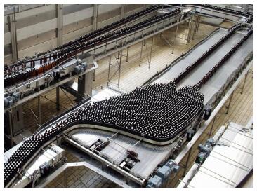
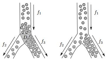
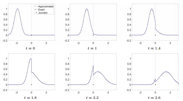
We introduce a macroscopic model for a network of conveyor belts with various speeds and capacities. In a different way from traffic flow models, the product densities are forced to move with a constant velocity unless they reach a maximal capacity and start to queue. This kind of dynamics is governed by scalar conservation laws consisting of a discontinuous flux function. We define appropriate coupling conditions to get well-posed solutions at intersections and provide a detailed description of the solution. Some numerical simulations are presented to illustrate and confirm the theoretical results for different network configurations.
Citation: Adriano Festa, Simone Göttlich, Marion Pfirsching. A model for a network of conveyor belts with discontinuous speed and capacity[J]. Networks and Heterogeneous Media, 2019, 14(2): 389-410. doi: 10.3934/nhm.2019016
We introduce a macroscopic model for a network of conveyor belts with various speeds and capacities. In a different way from traffic flow models, the product densities are forced to move with a constant velocity unless they reach a maximal capacity and start to queue. This kind of dynamics is governed by scalar conservation laws consisting of a discontinuous flux function. We define appropriate coupling conditions to get well-posed solutions at intersections and provide a detailed description of the solution. Some numerical simulations are presented to illustrate and confirm the theoretical results for different network configurations.

| [1] |
A scalar conservation law with discontinuous flux for supply chains with finite buffers. SIAM J. Appl. Math. (2011) 71: 1070-1087. 
|
| [2] |
A discrete hughes model for pedestrian flow on graphs. Netw. Heterog. Media (2017) 12: 93-112.
|
| [3] |
C. d'Apice, S. Göttlich, M. Herty and B. Piccoli, Modeling, Simulation, and Optimization of Supply Chains: A Continuous Approach, SIAM, 2010. doi: 10.1137/1.9780898717600
|
| [4] |
On the riemann problem for some discontinuous systems of conservation laws describing phase transitions. Commun. Pure Appl. Math. (2004) 3: 53-58.
|
| [5] |
Solutions to a scalar discontinuous conservation law in a limit case of phase transitions. J. Math. Fluid Mech. (2005) 7: 153-163.
|
| [6] |
Arbitrarily high-order accurate entropy stable essentially nonoscillatory schemes for systems of conservation laws. SIAM J. Numer. Anal. (2012) 50: 544-573.
|
| [7] | M. Garavello, K. Han and B. Piccoli, Models for Vehicular Traffic on Networks, volume 9, American Institute of Mathematical Sciences (AIMS), Springfield, MO, 2016. |
| [8] |
Conservation laws with discontinuous flux. Netw. Heterog. Media (2007) 2: 159-179.
|
| [9] | M. Garavello and B. Piccoli, Traffic Flow on Networks, volume 1, American Institute of Mathematical Sciences (AIMS), Springfield, MO, 2006. |
| [10] |
Discontinuous conservation laws for production networks with finite buffers. SIAM J. Appl. Math. (2013) 73: 1117-1138.
|
| [11] |
Existence of solution to supply chain models based on partial differential equation with discontinuous flux function. J. Math. Anal. Appl. (2013) 401: 510-517.
|
| [12] |
Convergence of a difference scheme for conservation laws with a discontinuous flux. SIAM J. Numer. Anal. (2000) 38: 681-698.
|
| [13] |
Riemann solver for a kinematic wave traffic model with discontinuous flux. J. Comput. Phys. (2013) 242: 1-23.
|
Figures(13) / Tables(1)
Adriano Festa, Simone Göttlich, Marion Pfirsching. A model for a network of conveyor belts with discontinuous speed and capacity[J]. Networks and Heterogeneous Media, 2019, 14(2): 389-410. doi: 10.3934/nhm.2019016


 DownLoad: