Mathematical modeling of mutated COVID-19 transmission with quarantine, isolation and vaccination

Fang Wang; Lianying Cao; Xiaoji Song; Fang Wang; Lianying Cao; Xiaoji Song

doi:10.3934/mbe.2022376

Mathematical Biosciences and Engineering

2022, Volume 19, Issue 8: 8035-8056. doi: 10.3934/mbe.2022376

Previous Article Next Article

Research article Special Issues

Mathematical modeling of mutated COVID-19 transmission with quarantine, isolation and vaccination

Department of Mathematics, Northeast Forestry University, Harbin 150040, China

Academic Editor: Pierre Magal

Received: 05 March 2022 Revised: 01 April 2022 Accepted: 23 May 2022 Published: 01 June 2022

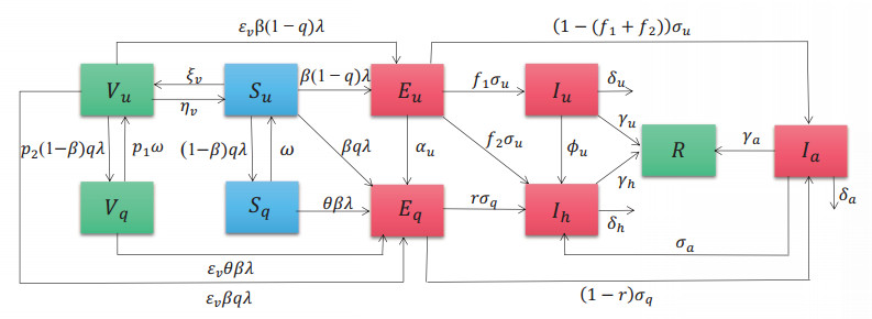
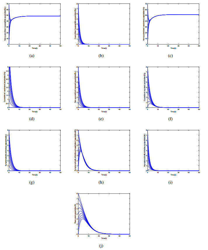
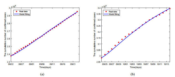
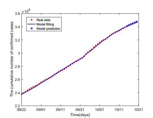
Multiple variants of SARS-CoV-2 have emerged but the effectiveness of existing COVID-19 vaccines against variants has been reduced, which bring new challenges to the control and mitigation of the COVID-19 pandemic. In this paper, a mathematical model for mutated COVID-19 with quarantine, isolation and vaccination is developed for studying current pandemic transmission. The basic reproduction number $ \mathscr{R}_{0} $ is obtained. It is proved that the disease free equilibrium is globally asymptotically stable if $ \mathscr{R}_{0} < 1 $ and unstable if $ \mathscr{R}_{0} > 1 $. And numerical simulations are carried out to illustrate our main results. The COVID-19 pandemic mainly caused by Delta variant in South Korea is analyzed by using this model and the unknown parameters are estimated by fitting to real data. The epidemic situation is predicted, and the prediction result is basically consistent with the actual data. Finally, we investigate several critical model parameters to access the impact of quarantine and vaccination on the control of COVID-19, including quarantine rate, quarantine effectiveness, vaccination rate, vaccine efficacy and rate of immunity loss.
- COVID-19,
- quarantine,
- isolation,
- vaccination,
- variants
Citation: Fang Wang, Lianying Cao, Xiaoji Song. Mathematical modeling of mutated COVID-19 transmission with quarantine, isolation and vaccination[J]. Mathematical Biosciences and Engineering, 2022, 19(8): 8035-8056. doi: 10.3934/mbe.2022376

Related Papers:

Abstract

Multiple variants of SARS-CoV-2 have emerged but the effectiveness of existing COVID-19 vaccines against variants has been reduced, which bring new challenges to the control and mitigation of the COVID-19 pandemic. In this paper, a mathematical model for mutated COVID-19 with quarantine, isolation and vaccination is developed for studying current pandemic transmission. The basic reproduction number $ \mathscr{R}_{0} $ is obtained. It is proved that the disease free equilibrium is globally asymptotically stable if $ \mathscr{R}_{0} < 1 $ and unstable if $ \mathscr{R}_{0} > 1 $. And numerical simulations are carried out to illustrate our main results. The COVID-19 pandemic mainly caused by Delta variant in South Korea is analyzed by using this model and the unknown parameters are estimated by fitting to real data. The epidemic situation is predicted, and the prediction result is basically consistent with the actual data. Finally, we investigate several critical model parameters to access the impact of quarantine and vaccination on the control of COVID-19, including quarantine rate, quarantine effectiveness, vaccination rate, vaccine efficacy and rate of immunity loss.

References

[1]	Q. Li, X. H. Guan, P. Wu, X. Y. Wang, L. Zhou, Y. Q. Tong, et al., Early transmission dynamics in Wuhan, China, of novel coronavirus–infected pneumonia, N. Engl. J. Med., 382 (2020), 1199–1207. https://doi.org/10.1056/NEJMoa2001316 doi: 10.1056/NEJMoa2001316
[2]	World Health Organization, WHO coronavirus disease (COVID-19) dashboard, 2022. Available from: https://covid19.who.int/.
[3]	C. C. John, V. Ponnusamy, S. K. Chandrasekaran, R. Nandakumar, A survey on mathematical, machine learning and deep learning models for COVID-19 transmission and diagnosis, IEEE Rev. Biomed. Eng., 15 (2021), 325–340. https://doi.org/10.1109/RBME.2021.3069213 doi: 10.1109/RBME.2021.3069213
[4]	Z. H. Yu, A. Sohail, T. A. Nofal, J. M. R. S. Tavares, Explainability of neural network clustering in interpreting the COVID-19 emergency data, Fractals, (2021). https://doi.org/10.1142/S0218348X22401223 doi: 10.1142/S0218348X22401223
[5]	Z. H. Yu, A. S. G. Abdel-Salam, A. Sohail, F. Alam, Forecasting the impact of environmental stresses on the frequent waves of COVID19, Nonlinear Dyn., 106 (2021), 1509–1523. https://doi.org/10.1007/s11071-021-06777-6 doi: 10.1007/s11071-021-06777-6
[6]	Z. H. Yu, R. Ellahi, A. Nutini, A. Sohail, S. M. Sait, Modeling and simulations of CoViD-19 molecular mechanism induced by cytokines storm during SARS-CoV2 infection, J. Mol. Liq., 327 (2021), 114863. https://doi.org/10.1016/j.molliq.2020.114863 doi: 10.1016/j.molliq.2020.114863
[7]	Z. H. Yu, H. X. Gao, D. Wang, A. A. Alnuaim, M. Firdausi, A. M. Mostafa, SEI$^{2}$RS malware propagation model considering two infection rates in cyber-physical systems, Physica A, 597 (2022), 127207. https://doi.org/10.1016/j.physa.2022.127207 doi: 10.1016/j.physa.2022.127207
[8]	Z. H. Yu, S. Lu, D. Wang, Z. W. Li, Modeling and analysis of rumor propagation in social networks, Inf. Sci., 580 (2021), 857–873. https://doi.org/10.1016/j.ins.2021.09.012 doi: 10.1016/j.ins.2021.09.012
[9]	N. Perra, Non-pharmaceutical interventions during the COVID-19 pandemic: A review, Phys. Rep., 913 (2021), 1–52. https://doi.org/10.1016/j.physrep.2021.02.001 doi: 10.1016/j.physrep.2021.02.001
[10]	C. N. Ngonghala, E. Iboi, S. Eikenberry, M. Scotch, C. R. MacIntyre, M. H. Bonds, et al., Mathematical assessment of the impact of non-pharmaceutical interventions on curtailing the 2019 novel Coronavirus, Math. Biosci., 325 (2020), 108364. https://doi.org/10.1016/j.mbs.2020.108364 doi: 10.1016/j.mbs.2020.108364
[11]	Z. H. Yu, R. Arif, M. A. Fahmy, A. Sohail, Self organizing maps for the parametric analysis of COVID-19 SEIRS delayed model, Chaos Solitons Fractals, 150 (2021), 111202. https://doi.org/10.1016/j.chaos.2021.111202 doi: 10.1016/j.chaos.2021.111202
[12]	M. Jeyanathan, S. Afkhami, F. Smaill, M. S. Miller, B. D. Lichty, Z. Xing, Immunological considerations for COVID-19 vaccine strategies, Nat. Rev. Immunol., 20 (2020), 615–632. https://doi.org/10.1038/s41577-020-00434-6 doi: 10.1038/s41577-020-00434-6
[13]	T. J. Bollyky, US COVID-19 vaccination challenges go beyond supply, Ann. Intern. Med., 174 (2021), 558–559. https://doi.org/10.7326/M20-8280 doi: 10.7326/M20-8280
[14]	E. A. Iboi, C. N. Ngonghala, A. B. Gumel, Will an imperfect vaccine curtail the COVID-19 pandemic in the US?, Infect. Dis. Model., 5 (2020), 510–524. https://doi.org/10.1016/j.idm.2020.07.006 doi: 10.1016/j.idm.2020.07.006
[15]	B. Huang, J. H. Wang, J. X. Cai, S. Q. Yao, P. K. S. Chan, T. H. Tam, et al., Integrated vaccination and physical distancing interventions to prevent future COVID-19 waves in Chinese cities, Nat. Hum. Behav., 5 (2021), 695–705. https://doi.org/10.1038/s41562-021-01063-2 doi: 10.1038/s41562-021-01063-2
[16]	Y. K. Zou, W. Yang, J. J. Lai, J. W. Hou, W. Lin, Vaccination and quarantine effect on COVID-19 transmission dynamics incorporating Chinese-Spring-Festival travel rush: Modeling and simulations, Bull. Math. Biol., 84 (2022), 1–19. https://doi.org/10.1007/s11538-021-00958-5 doi: 10.1007/s11538-021-00958-5
[17]	World Health Organization, Coronavirus disease (COVID-19): Variants of SARS-COV-2, 2022. Available from: https://www.who.int/emergencies/diseases/novel-coronavirus-2019/question-and-answers-hub/q-a-detail/coronavirus-disease-(covid-19)-variants-of-sars-cov-2.
[18]	World Health Organization, Coronavirus disease (COVID-19): Vaccines, 2022. Available from: https://www.who.int/emergencies/diseases/novel-coronavirus-2019/question-and-answers-hub/q-a-detail/coronavirus-disease-(covid-19)-vaccines.
[19]	T. T. Li, Y. M. Guo, Modeling and optimal control of mutated COVID-19 (Delta strain) with imperfect vaccination, Chaos Solitons Fractals, 156 (2022), 111825. https://doi.org/10.1016/j.chaos.2022.111825 doi: 10.1016/j.chaos.2022.111825
[20]	A. Truszkowska, L. Zino, S. Butail, E. Caroppo, Z. P. Jiang, A. Rizzo, et al., Predicting the effects of waning vaccine immunity against COVID-19 through high-resolution agent-based modeling, Adv. Theory Simul., (2022), 2100521. https://doi.org/10.1002/adts.202100521 doi: 10.1002/adts.202100521
[21]	V. Lakshmikantham, S. Leela, A. A. Martynyuk, Stability analysis of nonlinear systems, Marcel Dekker, Inc., New York and Basel, 1989. https://doi.org/10.1007/978-3-319-27200-9
[22]	P. Van den Driessche, J. Watmough, Reproduction numbers and sub-threshold endemic equilibria for compartmental models of disease transmission, Math. Biosci., 180 (2002), 29–48. https://doi.org/10.1016/S0025-5564(02)00108-6 doi: 10.1016/S0025-5564(02)00108-6
[23]	O. Diekmann, J. A. P. Heesterbeek, J. A. J. Metz, O. Diekmann, On the definition and the computation of the basic reproduction ratio $R_{0}$ in models for infectious diseases in heterogeneous populations, J. Math. Biol., 28 (1990), 365–382.
[24]	J. P. LaSalle, The stability of dynamical systems, Regional Conf. Ser. Appl. Math., SIAM, Philadelphia, 1976.
[25]	Central Disaster Management Headquarters of Korea, 2021. Available from: http://ncov.mohw.go.kr.
[26]	Our World in Data, 2021. Available from: https://ourworldindata.org/coronavirus#explore-the-global-situation.
[27]	Korea Disease Control and Prevention Agency, 2021. Available from: https://www.kdca.go.kr/index.es?sid=a2.
[28]	Central Disaster Management Headquarters of Korea, What is the criteria for releasing an asymptomatic person who tests positive for the virus from quarantine?, 2021. Available from: http://ncov.mohw.go.kr/en/faqBoardList.do?brdId=13&brdGubun=131&dataGubun=&ncvContSeq=&contSeq=&board_id=.
[29]	M. Zhang, J. P. Xiao, A. P. Deng, Y. T. Zhang, Y. L. Zhuang, T. Hu et al., Transmission dynamics of an outbreak of the COVID-19 Delta variant B. 1.617. 2–Guangdong Province, China, May–June 2021, China CDC Wkly, 3 (2021), 584–586. https://doi.org/10.46234/ccdcw2021.148 doi: 10.46234/ccdcw2021.148
[30]	M. Z. Yin, Q. W. Zhu, X. Lü, Parameter estimation of the incubation period of COVID-19 based on the doubly interval-censored data model, Nonlinear Dyn., 106 (2021), 1347–1358. https://doi.org/10.1007/s11071-021-06587-w doi: 10.1007/s11071-021-06587-w
[31]	N. Ferguson, D. Laydon, G. Nedjati-Gilani, N. Imai, K. Ainslie, M. Baguelin, et al., Report 9: Impact of non-pharmaceutical interventions (NPIs) to reduce COVID19 mortality and healthcare demand, Imperial College London, 10 (2020), 491–497. https://doi.org/10.25561/77482 doi: 10.25561/77482
[32]	S. M. Kissler, C. Tedijanto, E. Goldstein, Y. H. Grad, M. Lipsitch, Projecting the transmission dynamics of SARS-CoV-2 through the postpandemic period, Science, 368 (2020), 860–868. https://doi.org/10.1126/science.abb5793 doi: 10.1126/science.abb5793
[33]	O. Byambasuren, M. Cardona, K. Bell, J. Clark, M. L. McLaws, P. Glasziou, Estimating the extent of asymptomatic COVID-19 and its potential for community transmission: systematic review and meta-analysis, J. Assoc. Med. Microbiol. Infect. Dis. Can., 5 (2020), 223–234. https://doi.org/10.3138/jammi-2020-0030 doi: 10.3138/jammi-2020-0030
[34]	R. Y. Li, S. Pei, B. Chen, Y. M. Song, T. Zhang, W. Yang, et al., Substantial undocumented infection facilitates the rapid dissemination of novel coronavirus (SARS-CoV-2), Science, 368 (2020), 489–493. https://doi.org/10.1126/science.abb3221 doi: 10.1126/science.abb3221
[35]	SOUTH KOREA, Average Lifespan, The information of average lifespan in South Korea, 2021. Available from: https://m.naver.com/.
[36]	SOUTH KOREA, Population, The information of population in South Korea, 2021. Available from: https://m.naver.com/.
[37]	World Health Organization, WHO target product profiles for COVID-19 vaccines, 2021. Available from: https://www.who.int/publications/m/item/who-target-product-profiles-for-covid-19-vaccines.
[38]	Korea Disease Control and Prevention Agency, Are COVID-19 vaccinations effective, 2021. Available from: https://ncv.kdca.go.kr/menu.es?mid=a20102000000.
[39]	Central Disaster Management Headquarters of Korea, 2021. Available from: http://ncov.mohw.go.kr/tcmBoardList.do?brdId=3&brdGubun=.
[40]	Korea Disease Control and Prevention Agency, 2021. Available from: http://www.kdca.go.kr/board/board.es?mid=a20501010000&bid=0015.
[41]	Korea Disease Control and Prevention Agency, The outbreak and vaccination status of COVID-19 in Korea (8.23., as of 0: 00), 2021. Available from: https://www.kdca.go.kr/board/board.es?mid=a20501010000&bid=0015&list_no=716586&cg_code =&act=view&nPage=20.
[42]	B. Tang, X. Wang, Q. Li, N. L. Bragazzi, S. Y. Tang, Y. N. Xiao, et al., Estimation of the transmission risk of the 2019-nCoV and its implication for public health interventions, J. Clin. Med., 9 (2020), 462. https://doi.org/10.3390/jcm9020462 doi: 10.3390/jcm9020462

Reader Comments

Your name:*

Email:*
© 2022 the Author(s), licensee AIMS Press. This is an open access article distributed under the terms of the Creative Commons Attribution License (http://creativecommons.org/licenses/by/4.0)