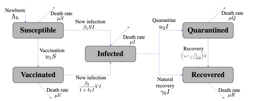
This study developed a deterministic transmission model for the coronavirus disease of 2019 (COVID-19), considering various factors such as vaccination, awareness, quarantine, and treatment resource limitations for infected individuals in quarantine facilities. The proposed model comprised five compartments: susceptible, vaccinated, quarantined, infected, and recovery. It also considered awareness and limited resources by using a saturated function. Dynamic analyses, including equilibrium points, control reproduction numbers, and bifurcation analyses, were conducted in this research, employing analytics to derive insights. Our results indicated the possibility of an endemic equilibrium even if the reproduction number for control was less than one. Using incidence data from West Java, Indonesia, we estimated our model parameter values to calibrate them with the real situation in the field. Elasticity analysis highlighted the crucial role of contact restrictions in reducing the spread of COVID-19, especially when combined with community awareness. This emphasized the analytics-driven nature of our approach. We transformed our model into an optimal control framework due to budget constraints. Leveraging Pontriagin's maximum principle, we meticulously formulated and solved our optimal control problem using the forward-backward sweep method. Our experiments underscored the pivotal role of vaccination in infection containment. Vaccination effectively reduces the risk of infection among vaccinated individuals, leading to a lower overall infection rate. However, combining vaccination and quarantine measures yields even more promising results than vaccination alone. A second crucial finding emphasized the need for early intervention during outbreaks rather than delayed responses. Early interventions significantly reduce the number of preventable infections, underscoring their importance.
Citation: C. K. Mahadhika, Dipo Aldila. A deterministic transmission model for analytics-driven optimization of COVID-19 post-pandemic vaccination and quarantine strategies[J]. Mathematical Biosciences and Engineering, 2024, 21(4): 4956-4988. doi: 10.3934/mbe.2024219
This study developed a deterministic transmission model for the coronavirus disease of 2019 (COVID-19), considering various factors such as vaccination, awareness, quarantine, and treatment resource limitations for infected individuals in quarantine facilities. The proposed model comprised five compartments: susceptible, vaccinated, quarantined, infected, and recovery. It also considered awareness and limited resources by using a saturated function. Dynamic analyses, including equilibrium points, control reproduction numbers, and bifurcation analyses, were conducted in this research, employing analytics to derive insights. Our results indicated the possibility of an endemic equilibrium even if the reproduction number for control was less than one. Using incidence data from West Java, Indonesia, we estimated our model parameter values to calibrate them with the real situation in the field. Elasticity analysis highlighted the crucial role of contact restrictions in reducing the spread of COVID-19, especially when combined with community awareness. This emphasized the analytics-driven nature of our approach. We transformed our model into an optimal control framework due to budget constraints. Leveraging Pontriagin's maximum principle, we meticulously formulated and solved our optimal control problem using the forward-backward sweep method. Our experiments underscored the pivotal role of vaccination in infection containment. Vaccination effectively reduces the risk of infection among vaccinated individuals, leading to a lower overall infection rate. However, combining vaccination and quarantine measures yields even more promising results than vaccination alone. A second crucial finding emphasized the need for early intervention during outbreaks rather than delayed responses. Early interventions significantly reduce the number of preventable infections, underscoring their importance.

| [1] | The World Health Organization (WHO), Coronavirus disease (covid-19) pandemic, 2023. Available from: https://www.who.int/europe/emergencies/situations/covid-19. |
| [2] | Centers for Disease Control and Prevention, Symptoms of covid-19, 2023. Available from: https://www.cdc.gov/coronavirus/2019-ncov/symptoms-testing/symptoms.html. |
| [3] | The World Health Organization (WHO), Indonesia situation of covid-19, 2023. Available from: https://covid19.who.int/region/searo/country/id. |
| [4] | Ministry of State Apparatus Utilization and Bureaucratic Reform, Indonesia (KEMENPANRI), Indonesia telah bergerak menuju endemi covid-199, 2023. Available from: https://www.menpan.go.id/site/berita-terkini/berita-daerah/indonesia-telah-bergerak-menuju-endemi-covid-19. |
| [5] | Communication Team of the National Committee for Handling Corona Virus Disease 2019 (Covid-19) and National Economic Recovery, Indonesia, Waspadai komorbid, salah satu faktor risiko yang memperparah gejala covid-19, 2022. Available from: https://covid19.go.id/artikel/2022/02/15/waspadai-komorbid-salah-satu-faktor-risiko-yang-memperparah-gejala-covid-19. |
| [6] | The Ministry of Health Republic Indonesia (KEMENKES RI), Covid 19 update, 2023. Available from: https://www.mayoclinic.org/diseases conditions/coronavirus/in-depth/herd-immunity-and coronavirus. |
| [7] |
K. Cardwell, B. Clyne, N. Broderick, B. Tyner, G. Masukume, L. Larkin, et al., Lessons learnt from the covid-19 pandemic in selected countries to inform strengthening of public health systems: a qualitative study, Public Health, 225 (2023), 343–352. https://doi.org/10.1016/j.puhe.2023.10.024 doi: 10.1016/j.puhe.2023.10.024

|
| [8] |
F. M. Ekawati, M. Muchlis, N. G. Iturrieta-Guaita, D. A. D. Putri, Recommendations for improving maternal health services in indonesian primary care under the covid-19 pandemic: Results of a systematic review and appraisal of international guidelines, Sex. Reprod. Healthcare, 35 (2023), 100811. https://doi.org/10.1016/j.srhc.2023.100811 doi: 10.1016/j.srhc.2023.100811
|
| [9] |
A. Rupp, P. Limpaphayom, Benefits of corporate social responsibility during a pandemic: Evidence from stock price reaction to covid-19 related news, Res. Int. Bus. Finance, 68 (2024), 102169. https://doi.org/10.1016/j.ribaf.2023.102169 doi: 10.1016/j.ribaf.2023.102169
|
| [10] |
I. D. Selvi, Online learning and child abuse: the covid-19 pandemic impact on work and school from home in indonesia, Heliyon, 8 (2022), e08790. https://doi.org/10.1016/j.heliyon.2022.e08790 doi: 10.1016/j.heliyon.2022.e08790
|
| [11] |
R. Banerjee, R. K. Biswas, Fractional optimal control of compartmental sir model of covid-19: Showing the impact of effective vaccination, IFAC-PapersOnLine, 55 (2022), 616–622. https://doi.org/10.1016/j.ifacol.2022.04.101 doi: 10.1016/j.ifacol.2022.04.101
|
| [12] |
M. L. Diagne, H. Rwezaura, S. Y. Tchoumis, J. M. Tchuenche, A mathematical model of covid-19 with vaccination and treatment, Comput. Math. Methods Med., 2021 (2021), 1250129. https://doi.org/10.1155/2021/1250129 doi: 10.1155/2021/1250129
|
| [13] |
J. N. Paul, I. S. Mbalawata, S. S. Mirau, L. Masandawa, Mathematical modeling of vaccination as a control measure of stress to fight covid-19 infections, Chaos, Solitons Fractals, 166 (2023), 112920. https://doi.org/10.1016/j.chaos.2022.112920 doi: 10.1016/j.chaos.2022.112920
|
| [14] |
B. Yang, Z. Yu, Y. Cai, The impact of vaccination on the spread of covid-19: Studying by a mathematical model, Physica A, 590 (2022), 126717. https://doi.org/10.1016/j.physa.2021.126717 doi: 10.1016/j.physa.2021.126717
|
| [15] |
A. Ayalew, M. Yezbalew, T. Tilahun, T. Tesfa, Mathematical model and analysis on the impacts of vaccination and treatment in the control of the covid-19 pandemic with optimal control, J. Appl. Math., 2023 (2023), 8570311. https://doi.org/10.1155/2023/8570311 doi: 10.1155/2023/8570311
|
| [16] |
C. W. Chukwu, R. T. Alqahtani, F. F. Herdicho, A pontryagin's maximum principle and optimal control model with cost-effectiveness analysis of the covid-19 epidemic, Decis. Anal. J., 8 (2023), 100273. https://doi.org/10.1016/j.dajour.2023.100273 doi: 10.1016/j.dajour.2023.100273
|
| [17] |
S. Bhatter, K. Jangid, A. Abidemi, K. M. Owolabi, S. D. Purohit, A new fractional mathematical model to study the impact of vaccination on covid-19 outbreaks, Decis. Anal. J., 6 (2023), 100156. https://doi.org/10.1016/j.dajour.2022.100156 doi: 10.1016/j.dajour.2022.100156
|
| [18] |
C. Xu, Y. Yu, G. Ren, Y. Sun, X. Si, Stability analysis and optimal control of a fractional-order generalized seir model for the covid-19 pandemic, Appl. Math. Comput., 457 (2023), 128210. https://doi.org/10.1016/j.amc.2023.128210 doi: 10.1016/j.amc.2023.128210
|
| [19] |
C. M. Wachira, G. O. Lawi, L. O. Omondi, Travelling wave analysis of a diffusive covid-19 model, J. Appl. Math., 2022 (2022), 60522274. https://doi.org/10.1155/2022/6052274 doi: 10.1155/2022/6052274
|
| [20] |
B. Barnes, I. Takyi, B. E. Owusu, F. Ohene Boateng, A. Saahene, E. Saarah Baidoo, et al., Mathematical modelling of the spatial epidemiology of covid-19 with different diffusion coefficients, Int. J. Differ. Equations, 2022, 7563111. https://doi.org/10.1155/2022/7563111 doi: 10.1155/2022/7563111
|
| [21] |
A. El Koufi, N. El Koufi, Stochastic differential equation model of covid-19: Case study of pakistan, Results Phys., 34 (2022), 105218. https://doi.org/10.1016/j.rinp.2022.105218 doi: 10.1016/j.rinp.2022.105218
|
| [22] |
M. Pajaro, N. M. Fajar, A. A. Alonso, I. Otero-Muras, Stochastic sir model predicts the evolution of covid-19 epidemics from public health and wastewater data in small and medium-sized municipalities: A one year study, Chaos, Solitons Fractals, 164 (2022), 112671. https://doi.org/10.1016/j.chaos.2022.112671 doi: 10.1016/j.chaos.2022.112671
|
| [23] |
V. V. Khanna, K. Chadaga, N. Sampathila, R. Chadaga, A machine learning and explainable artificial intelligence triage-prediction system for covid-19, Decis. Anal. J., 7 (2023), 100246. https://doi.org/10.1016/j.dajour.2023.100246 doi: 10.1016/j.dajour.2023.100246
|
| [24] |
K. Moulaei, M. Shanbehzadeh, Z. Mohammadi-Taghiabad, H. Kazemi-Arpanahi, Comparing machine learning algorithms for predicting covid-19 mortality, BMC Med. Inf. Decis. Making, 22 (2022), 1–12. https://doi.org/10.1186/s12911-021-01742-0 doi: 10.1186/s12911-021-01742-0
|
| [25] |
D. Aldila, S. H. Khoshnaw, E. Safitri, Y. R. Anwar, A. R. Bakry, B. M. Samiadji, et al., A mathematical study on the spread of covid-19 considering social distancing and rapid assessment: the case of jakarta, indonesia, Chaos Solitons Fractals, 139 (2020), 110042. https://doi.org/10.1016/j.chaos.2020.110042 doi: 10.1016/j.chaos.2020.110042
|
| [26] |
J. L. Gevertz, J. M. Greene, C. H. Sanchez-Tapia, E. D. Sontag, A novel covid-19 epidemiological model with explicit susceptible and asymptomatic isolation compartments reveals unexpected consequences of timing social distancing, J. Theor. Biol., 510 (2021), 110539. https://doi.org/10.1016/j.jtbi.2020.110539 doi: 10.1016/j.jtbi.2020.110539
|
| [27] |
I. A. Arik, H. K. Sari, S. I. Araz, Numerical simulation of covid-19 model with integer and non-integer order: The effect of environment and social distancing, Results Phys., 51 (2023), 106725. https://doi.org/10.1016/j.rinp.2023.106725 doi: 10.1016/j.rinp.2023.106725
|
| [28] |
S. Saharan, C. Tee, A covid-19 vaccine effectiveness model using the susceptible-exposed-infectious-recovered model, Healthcare Anal., 4 (2023), 100269. https://doi.org/10.1016/j.health.2023.10026 doi: 10.1016/j.health.2023.10026
|
| [29] |
A. I. Alaje, M. O. Olayiwola, A fractional-order mathematical model for examining the spatiotemporal spread of covid-19 in the presence of vaccine distribution, Healthcare Anal., 4 (2023), 100230. https://doi.org/10.1016/j.health.2023.100230 doi: 10.1016/j.health.2023.100230
|
| [30] |
R. Pino, V. M. Mendoza, E. A. Enriques, A. C. Velasco, R. Mendoza, An optimization model with simulation for optimal regional allocation of covid-19 vaccines, Healthcare Anal., 4 (2023), 100244. https://doi.org/10.1016/j.health.2023.100244 doi: 10.1016/j.health.2023.100244
|
| [31] |
O. J. Watson, G. Barnsley, J. Toor, A. B. Hogan, P. Winskill, A. C. Ghani, Global impact of the first year of covid-19 vaccination: a mathematical modelling study, Lancet Infect. Dis., 22 (2022), 1293–1302. https://doi.org/10.1016/S1473-3099(22)00320-6 doi: 10.1016/S1473-3099(22)00320-6
|
| [32] |
A. K. Paul, M. A. Kuddus, Mathematical analysis of a covid-19 model with double dose vaccination in bangladesh, Results Phys., 35 (2022), 105392. https://doi.org/10.1016/j.rinp.2022.105392 doi: 10.1016/j.rinp.2022.105392
|
| [33] |
O. I. Idisi, T. T. Yusuf, K. M. Owolabi, B. A. Ojokoh, A bifurcation analysis and model of covid-19 transmission dynamics with post-vaccination infection impact, Healthcare Anal., 3 (2023), 100157. https://doi.org/10.1016/j.health.2023.100157 doi: 10.1016/j.health.2023.100157
|
| [34] |
I. Ul Haq, N. Ullah, N. Ali, K. S. Nisar, A new mathematical model of covid-19 with quarantine and vaccination, Mathematics, 11 (2022), 142. https://doi.org/10.3390/math11010142 doi: 10.3390/math11010142
|
| [35] |
D. S. A. A. Reza, M. N. Billah, S. S. Shanta, Effect of quarantine and vaccination in a pandemic situation: A mathematical modelling approach, J. Math. Anal. Model., 2 (2021), 77–81. https://doi.org/10.48185/jmam.v2i3.318 doi: 10.48185/jmam.v2i3.318
|
| [36] |
Y. Gu, S. Ullah, M. A. Khan, Mathematical modeling and stability analysis of the covid-19 with quarantine and isolation, Results Phys., 34 (2022), 105284. https://doi.org/10.1016/j.rinp.2022.105284 doi: 10.1016/j.rinp.2022.105284
|
| [37] |
F. Wu, X. Liang, J. Lein, Modelling covid-19 epidemic with confirmed cases-driven contact tracing quarantine, Infect. Dis. Modell., 8 (2023), 415–426. https://doi.org/10.1016/j.idm.2023.04.001 doi: 10.1016/j.idm.2023.04.001
|
| [38] |
A. K. Saha, S. Saha, C. N. Podder, Effect of awareness, quarantine and vaccination as control strategies on covid-19 with co-morbidity and re-infection, Infect. Dis. Modell., 7 (2022), 660–689. https://doi.org/10.1016/j.idm.2022.09.004 doi: 10.1016/j.idm.2022.09.004
|
| [39] |
S. S. Musa, S. Queshi, S. Zhao, A. Yusuf, U. T. Mustapha, D. He, Mathematical modeling of covid-19 epidemic with effect of awareness programs, Infect. Dis. Modell., 6 (2021), 448–460. https://doi.org/10.1016/j.idm.2021.01.012 doi: 10.1016/j.idm.2021.01.012
|
| [40] |
A. A. Anteneh, Y. M. Bazazaw, S. Palanisam, Mathematical model and analysis on the impact of awareness campaign and asymptomatic human immigrants in the transmission of covid-19, Biomed Res. Int., 2022 (2022), 6260262. https://doi.org/10.1155/2022/6260262 doi: 10.1155/2022/6260262
|
| [41] |
M. A. Balya, B. O. Dewi, F. I. Lestari, G. Ratu, H. Rosuliyana, T. Windyhani, et al., Investigating the impact of social awareness and rapid test on a covid-19 transmission model, Commun. Biomathematical Sci., 4 (2021), 46–64. https://doi.org/10.5614/cbms.2021.4.1.5 doi: 10.5614/cbms.2021.4.1.5
|
| [42] |
A. K. Srivastav, M. Gosh, S. S. Bandekar, Modeling of covid-19 with limited public health resources: a comparative study of three most affected countries, Eur. Phys. J. Plus, 136 (2021), 359. https://doi.org/10.1140/epjp/s13360-021-01333-y doi: 10.1140/epjp/s13360-021-01333-y
|
| [43] |
U. M. Rifanti, A. R. Dewi, N. Nurlaili, S. T. Hapsari, Model matematika covid-19 dengan sumber daya pengobatan yang terbatas, J. Math. Appl., 18 (2021), 23–36. https://doi.org/10.12962/limits.v18i1.8207 doi: 10.12962/limits.v18i1.8207
|
| [44] |
S. Cakan, Dynamic analysis of a mathematical model with health care capacity for covid-19 pandemic, Chaos, Solitons, Fractals, 139 (2020), 110033. https://doi.org/10.1016/j.chaos.2020.110033 doi: 10.1016/j.chaos.2020.110033
|
| [45] |
I. I. Oke, Y. T. Oyebo, O. F. Fakoya, V. S. Benson, Y. T. Tunde, A mathematical model for covid-19 disease transmission dynamics with impact of saturated treatment: Modeling, analysis and simulation, Open Access Lib. J., 8 (2021), 1–20. https://doi.org/10.4236/oalib.1107332 doi: 10.4236/oalib.1107332
|
| [46] |
M. Elhia, L. Boujallal, M. Alkama, O. Balatif, M. Rachik, Set-valued control approach applied to a covid-19 model with screening and saturated treatment function, Complexity, 2020 (2020), 9501028. https://doi.org/10.1155/2020/9501028 doi: 10.1155/2020/9501028
|
| [47] |
J. K. Ghosh, S. K. Bhiswas, S. Sarkar, U. Ghosh, Mathematical modelling of covid-19: A case study of italy, Math. Comput. Simul., 194 (2022), 1–18. https://doi.org/10.1016/j.matcom.2021.11.008 doi: 10.1016/j.matcom.2021.11.008
|
| [48] |
R. T. Alqahtani, A. Ajbar, Study of dynamics of a covid-19 model for saudi arabia with vaccination rate, saturated treatment function and saturated incidence rate, Mathematics, 9 (2021), 3134. https://doi.org/10.3390/math9233134 doi: 10.3390/math9233134
|
| [49] |
I. Ali, S. U. Khan, Dynamics and simulations of stochastic covid 19 epidemic model using legendre spectral collocation method, AIMS Math., 8 (2023), 4220–4236. https://doi.org/10.3934/math.2023210 doi: 10.3934/math.2023210
|
| [50] |
S. S. Chaharborj, S. S. Chaharborj, J. H. Asl, P. S. Phang, Controlling pandemic covid-19 using optimal control theory, Results Phys., 26 (2021), 104311. https://doi.org/10.1016/j.rinp.2021.104311 doi: 10.1016/j.rinp.2021.104311
|
| [51] |
R. P. Kumar, S. Basu, P. K. Santra, D. Ghosh, G. S. Mahapatra, Optimal control design incorporating vaccination and treatment on six compartment pandemic dynamical system, Results Control Optim., 7 (2022), 100115. https://doi.org/10.1016/j.rico.2022.100115 doi: 10.1016/j.rico.2022.100115
|
| [52] |
T. Li, Y. Guo, Optimal control and cost-effectiveness analysis of a new covid-19 model for omicron strain, Physica A, 606 (2022), 128134. https://doi.org/10.1016/j.physa.2022.128134 doi: 10.1016/j.physa.2022.128134
|
| [53] |
A. Bilgram, P. G. Jensen, K. Y. Jørgensen, K. G. Larsen, M. Mikučionis, M. Muñiz, et al., An investigation of safe and near-optimal strategies for prevention of covid-19 exposure using stochastic hybrid models and machine learning, Decis. Anal. J., 5 (2022), 100141. https://doi.org/10.1016/j.dajour.2022.100141 doi: 10.1016/j.dajour.2022.100141
|
| [54] |
M. S. Khatun, S. Das, P. Das, Dynamics and control of an sitr covid-19 model with awareness and hospital bed dependency, Chaos, Solitons Fractals, 175 (2023), 114010. https://doi.org/10.1016/j.chaos.2023.114010 doi: 10.1016/j.chaos.2023.114010
|
| [55] | Mayo Clinic, Herd immunity and covid-19: What you need to know, 2023. Available from: https://www.mayoclinic.org/diseases conditions/coronavirus/in-depth/herd-immunity-and coronavirus. |
| [56] | D. K. A. Mannan, K. M. Farhana, Knowledge, attitude and acceptance of a covid‐19 vaccine: a global cross‐sectional study, Int. Res. J. Bus. Social Sci., 6 (2020), 1–23. |
| [57] |
S. M. Saeied, M. M. Saeied, I. A. Kabbash, S. Abdo, Vaccine hesitancy: beliefs and barriers associated with covid‐19 vaccination among egyptian medical students, J. Med. Virol., 93 (2021), 4280–4291. https://doi.org/10.1002/jmv.26910 doi: 10.1002/jmv.26910
|
| [58] |
M. O. Elgendy, M. E. A. Abdelrahim, Public awareness about coronavirus vaccine, vaccine acceptance, and hesitancy, J. Med. Virol., 93.(2021), 6535–6543. https://doi.org/10.1002/jmv.27199 doi: 10.1002/jmv.27199
|
| [59] |
S. Funk, E. Gilad, C. Watkins, V. A. A. Jansen, The spread of awareness and its impact on epidemic outbreaks, Proc. Natl. Acad. Sci., 106 (2009), 6872–6877. https://doi.org/10.1073/pnas.0810762106 doi: 10.1073/pnas.0810762106
|
| [60] |
G. Kelly, S. Petti, N. Noah, Covid-19, non-covid-19 and excess mortality rates not comparable across countries, Epidemiol. Infect., 149 (2021), e176. https://doi.org/10.1017/S0950268821001850 doi: 10.1017/S0950268821001850
|
| [61] |
S. Nourazari, S. R. Davis, R. Granovsky, R. Austin, D. J. Straff, J. W. Joseph, L. D. Sanchez, Decreased hospital admissions through emergency departments during the covid-19 pandemic, Am. J. Emerg. Med., 42 (2021), 203–210. https://doi.org/10.1016/j.ajem.2020.11.029 doi: 10.1016/j.ajem.2020.11.029
|
| [62] | Statistics Center of West Java Province (BPS), Jumlah penduduk menurut kabupaten/kota (jiwa), 2018-2020, 2023. Available from: https://jabar.bps.go.id/indicator/12/133/1/jumlah-penduduk-menurut-kabupaten-kota.html. |
| [63] |
A. Abidemi, J. O. Akanni, O. D. Makinde, A non-linear mathematical model for analysing the impact of covid-19 disease on higher education in developing countries, Healthcare Anal., 3 (2023), 100193. https://doi.org/10.1016/j.health.2023.100193 doi: 10.1016/j.health.2023.100193
|
| [64] |
E. A. Iboi, O. Sharomi, C. N. Ngonghala, A. B. Gumel, Mathematical modeling and analysis of covid-19 pandemic in nigeria, Math. Biosci. Eng., 17 (2020), 7192–7220. https://doi.org/10.3934/mbe.2020369 doi: 10.3934/mbe.2020369
|
| [65] | Statistics Center of West Java Province (BPS), [komponen ipg] usia harapan hidup 2020-2022, 2023. Available from: https://jabar.bps.go.id/indicator/40/185/1/-komponen-ipg-usia-harapan-hidup-.html. |
| [66] |
S. Olaniyi, O. S. Obabiyi, K. O. Okosun, A. T. Oladipo, S. O. Adewale, Athematical modelling and optimal cost-effective control of covid-19 transmission dynamics, Eur. Phys. J. Plus, 135 (2021), 1–20. https://doi.org/10.1140/epjp/s13360-020-00954-z doi: 10.1140/epjp/s13360-020-00954-z
|
| [67] |
A. Abate, A. Tiwari, S. Sastrys, Box invariance in biologically-inspired dynamical systems, Automatica, 45 (2009), 1601–1610. https://doi.org/10.1016/j.automatica.2009.02.028 doi: 10.1016/j.automatica.2009.02.028
|
| [68] |
P. Taylan, G. W. Weber, L. Liu, F. Yerlika-Ozkurt, On the foundations of parameter estimation for generalized partial linear models with b-splines and continuous optimization, Comput. Math. Appl., 60 (2010), 134–143. https://doi.org/10.1016/j.camwa.2010.04.040 doi: 10.1016/j.camwa.2010.04.040
|
| [69] |
A. A. Tappe, M. Schulze, R. Schenkendorf, Neural odes and differential flatness for total least squares parameter estimation, IFAC-PapersOnLine, 55 (2020), 421–426. https://doi.org/10.1016/j.ifacol.2022.09.131 doi: 10.1016/j.ifacol.2022.09.131
|
| [70] |
O. Aydogmuz, T. Ali Hakan, A modified multiple shooting algorithm for parameter estimation in odes using adjoint sensitivity analysis, Appl. Math. Comput., 390 (2021), 125644. https://doi.org/10.1016/j.amc.2020.125644 doi: 10.1016/j.amc.2020.125644
|
| [71] |
S. Khalilpourazari, H. Hashemi Doulabi, A. O. Ciftcioglu, G. W. Weber, Gradient-based grey wolf optimizer with gaussian walk: Application in modelling and prediction of the covid-19 pandemic, Expert Syst. Appl., 177 (2021), 114920. https://doi.org/10.1016/j.eswa.2021.114920 doi: 10.1016/j.eswa.2021.114920
|
| [72] |
P. Driesche, J. Watmough, Reproduction numbers and sub-threshold endemic equilibria for compartmental models of disease transmissions, Math. Biosci., 180 (2002), 29–48. https://doi.org/10.1016/S0025-5564(02)00108-6 doi: 10.1016/S0025-5564(02)00108-6
|
| [73] | M. Martcheva, An Introduction to Mathematical Epidemiology, Springer, Berlin, Germany, 2015. |
| [74] |
C. Castillo–Chavez, B. Song, Dynamical models of tuberculosis and their applications, Math. Biosci. Eng., 1 (2024), 361–404. https://doi.org/10.3934/mbe.2004.1.361 doi: 10.3934/mbe.2004.1.361
|
| [75] | S. Leinhart, J. T. Workman, Optimal Control Applied to Biological Models, Taylor & Francis Group, CRC press, Boca Raton, Florida, USA, 2007. |
| [76] |
D. Aldila, Cost-effectiveness and backward bifurcation analysis on covid-19 transmission model considering direct and indirect transmission, Commun. Math. Biol. Neurosci., 2020 (2020), 49. https://doi.org/10.28919/cmbn/4779 doi: 10.28919/cmbn/4779
|
| [77] |
D. Aldila, A. Nadya, Fatmawati, F. F. Herdicho, M. Z. Ndii, C. W. Chukwu, Optimal control of pneumonia transmission model with seasonal factor: Learning from jakarta incidence data, Heliyon, 9 (2023), e18096. https://doi.org/10.1016/j.heliyon.2023.e18096 doi: 10.1016/j.heliyon.2023.e18096
|
| [78] |
D. Aldila, M. Angelina, Optimal control problem and backward bifurcation on malaria transmission with vector bias, Heliyon, 7 (2021), e06824. https://doi.org/10.1016/j.heliyon.2021.e06824 doi: 10.1016/j.heliyon.2021.e06824
|
| [79] |
D. Aldila, Optimal control for dengue eradication program under the media awareness effect, Int. J. Nonlinear Sci. Numer. Simul., 24 (2023), 95–122. https://doi.org/10.1515/ijnsns-2020-0142 doi: 10.1515/ijnsns-2020-0142
|
| [80] |
O. Sharomi, C. N. Podder, A. B, Gumel, B. Song, Mathematical analysis of the transmission dynamics of hiv/tb co-infection in the presence of treatment, Math. Biosci. Eng., 5 (2008), 145–174. https://doi.org/10.3934/mbe.2008.5.145 doi: 10.3934/mbe.2008.5.145
|
| [81] |
E. H. Elbasha, C. N. Podder, A. B. Gumel, Analyzing the dynamics of an sirs vaccination model with waning natural and vaccine-induced immunity, Nonlinear Anal. Real World Appl., 12 (2011), 2692–2705. https://doi.org/10.1016/j.nonrwa.2011.03.015 doi: 10.1016/j.nonrwa.2011.03.015
|
| [82] |
A. B. Gumel, Causes of backward bifurcations in some epidemiological models, J. Math. Anal. Appl., 395 (2012), 355–365. https://doi.org/10.1016/j.jmaa.2012.04.077 doi: 10.1016/j.jmaa.2012.04.077
|
| [83] |
D. Aldila, J. P. Chavez, K. P. Wijaya, N. C. Ganegoda, G. M. Simorangkir, H. Tasman, et al., A tuberculosis epidemic model as a proxy for the assessment of the novel m72/as01e vaccine, Commun. Nonlinear Sci. Numer. Simul., 120 (2023), 107162. https://doi.org/10.1016/j.cnsns.2023.107162 doi: 10.1016/j.cnsns.2023.107162
|
| [84] |
K. Erik, W. Gerhard-Wilhelm, T. E. Babaee, Foundations of semialgebraic gene-environment networks, J. Dyn. Games, 7 (2020), 253–268. https://doi.org/10.3934/jdg.2020018 doi: 10.3934/jdg.2020018
|
| [85] |
S. Belen, E. Kropat, W. Gerhard-Wilhelm, On the classical maki–thompson rumour model in continuous time, Cent. Eur. Oper. Res., 19 (2011), 1–17. https://doi.org/10.1016/j.jmaa.2015.06.054 doi: 10.1016/j.jmaa.2015.06.054
|
| [86] | E. Savku, A stochastic control approach for constrained stochastic differential games with jumps and regimes, preprint, arXiv: 2301.12921. https://doi.org/10.48550/arXiv.2301.12921 |
Figures(10) / Tables(4)

C. K. Mahadhika, Dipo Aldila. A deterministic transmission model for analytics-driven optimization of COVID-19 post-pandemic vaccination and quarantine strategies[J]. Mathematical Biosciences and Engineering, 2024, 21(4): 4956-4988. doi: 10.3934/mbe.2024219


 DownLoad: