We developed a three-dimensional Filippov piecewise-smooth population system characterizing aphid–ladybug–ant interactions, in which a threshold-based switching function describes the transition of aphids between pure reproduction and honeydew-excreting ant-recruitment strategies. In conventional numerical simulations of ecological models, sustained oscillations are often identified directly as steady-state limit cycles. Within the framework of non-smooth dynamical systems, the sliding dynamics, equilibrium classification, and stability of the model were analyzed. Time-series simulations, maximum Lyapunov exponent scans, and semi-logarithmic amplitude-decay analysis revealed that the long-lasting damped oscillations of the system are long transients rather than genuine limit cycles, which can be easily misjudged as steady-state oscillations under finite simulation time. The system exhibited monostable and bistable behaviors within the parameter domains examined, and the long transients were jointly induced by the weak stability of equilibria and the geometric constraints of the piecewise switching structure; the threshold switching, rather than any adaptive optimization, shaped the transient population dynamics. These findings highlight the distinction between transient evolution and genuine steady-state behavior in threshold-regulated ecosystems and provide reliable references for the numerical identification of such dynamics.
Citation: Zheqi Tao, Yi Yang, Changcheng Xiang. Long-transient behaviors and dynamical misjudgment in a Filippov piecewise-smooth population model[J]. AIMS Mathematics, 2026, 11(11): 36356-36378. doi: 10.3934/math.20261407
We developed a three-dimensional Filippov piecewise-smooth population system characterizing aphid–ladybug–ant interactions, in which a threshold-based switching function describes the transition of aphids between pure reproduction and honeydew-excreting ant-recruitment strategies. In conventional numerical simulations of ecological models, sustained oscillations are often identified directly as steady-state limit cycles. Within the framework of non-smooth dynamical systems, the sliding dynamics, equilibrium classification, and stability of the model were analyzed. Time-series simulations, maximum Lyapunov exponent scans, and semi-logarithmic amplitude-decay analysis revealed that the long-lasting damped oscillations of the system are long transients rather than genuine limit cycles, which can be easily misjudged as steady-state oscillations under finite simulation time. The system exhibited monostable and bistable behaviors within the parameter domains examined, and the long transients were jointly induced by the weak stability of equilibria and the geometric constraints of the piecewise switching structure; the threshold switching, rather than any adaptive optimization, shaped the transient population dynamics. These findings highlight the distinction between transient evolution and genuine steady-state behavior in threshold-regulated ecosystems and provide reliable references for the numerical identification of such dynamics.

| [1] |
E. Diehl-Fleig, E. Diehl, Interactions among attending ants, brown-citrus aphids, and ladybugs in plants of Citrus sinensis, Neotrop. Biol. Conserv., 13 (2018), 161–170. http://dx.doi.org/10.4013/nbc.2018.132.08 doi: 10.4013/nbc.2018.132.08
|
| [2] |
Y. Lv, H. Wang, J. Ding, Q. Zhu, Dynamic analysis of a stochastic three species predator-prey model with intraguild predation and predator-switching, Commun. Nonlinear Sci., 157 (2026), 109748. http://dx.doi.org/10.1016/j.cnsns.2026.109748 doi: 10.1016/j.cnsns.2026.109748
|
| [3] |
Y. Wang, Z. Shen, L. Gao, X. Ma, Global analysis of a wheat aphid-ladybug model with age structure, J. Biomath., 22 (2007), 59–66. |
| [4] |
B. Stadler, A. F. G. Dixon, Ecology and evolution of aphid-ant interactions, Annu. Rev. Ecol. Evol. Syst., 36 (2005), 345–372. http://dx.doi.org/10.1146/annurev.ecolsys.36.091704.175531 doi: 10.1146/annurev.ecolsys.36.091704.175531
|
| [5] |
M. D. Bernardo, C. J. Budd, A. R. Champneys, P. Kowalczyk, Piecewise-smooth dynamical systems: Theory and applications, London: Springer, 2008. https://doi.org/10.1007/978-1-84628-708-4 |
| [6] |
A. F. Filippov, Differential equations with discontinuous righthand sides, Dordrecht: Springer, 1988. https://doi.org/10.1007/978-94-015-7793-9 |
| [7] |
Z. Zhang, R. Yang, Dynamical analysis of a reaction–diffusion Filippov food chain model with threshold control, Phys. D, 496 (2026), 135325. http://dx.doi.org/10.1016/j.physd.2026.135325 doi: 10.1016/j.physd.2026.135325
|
| [8] |
H. Zhou, S. Tang, Complex dynamics and sliding bifurcations of the Filippov Lorenz–Chen system, Int. J. Bifurcation Chaos, 32 (2022), 2250182. http://dx.doi.org/10.1142/S0218127422501826 doi: 10.1142/S0218127422501826
|
| [9] |
A. Hastings, Transient dynamics and persistence of ecological systems, Ecol. Lett., 4 (2001), 215–220. http://dx.doi.org/10.1046/j.1461-0248.2001.00220.x doi: 10.1046/j.1461-0248.2001.00220.x
|
| [10] |
D. Rockwell, E. Naudascher, Self-sustained oscillations of impinging free shear layers, Annu. Rev. Fluid Mech., 11 (1979), 67–94. http://dx.doi.org/10.1146/annurev.fl.11.010179.000435 doi: 10.1146/annurev.fl.11.010179.000435
|
| [11] |
V. D. Pechuk, T. S. Krasnopolskaya, E. D. Pechuk, Maximum Lyapunov exponent calculation, In: 14th Chaotic modeling and simulation international conference, 2022,327–335. http://dx.doi.org/10.1007/978-3-030-96964-6_22 |
| [12] |
J. H. Dirks, V. Dürr, Biomechanics of the stick insect antenna: Damping properties and structural correlates of the cuticle, J. Mech. Behav. Biomed. Mater., 4 (2011), 2031–2042. http://dx.doi.org/10.1016/j.jmbbm.2011.07.002 doi: 10.1016/j.jmbbm.2011.07.002
|
| [13] |
M. Forti, B. Garay, M. Koller, L. Pancioni, An experimental study on long transient oscillations in cooperative CNN rings, In: IEEE International workshop on cellular nanoscale networks and their applications (CNNA), 2012. http://dx.doi.org/10.1109/CNNA.2012.6331410 |
| [14] |
A. Rougirel, Convergence to steady state and attractors for doubly nonlinear equations, J. Math. Anal. Appl., 339 (2008), 281–294. http://dx.doi.org/10.1016/j.jmaa.2007.06.028 doi: 10.1016/j.jmaa.2007.06.028
|
| [15] |
S. Tang, J. Liang, Y. Xiao, R. A. Cheke, Sliding bifurcations of Filippov two stage pest control models with economic thresholds, SIAM J. Appl. Math., 72 (2012), 1061–1080. http://dx.doi.org/10.1137/110847020 doi: 10.1137/110847020
|
| [16] |
Y. Kuznetsov, S. Rinaldi, A. Gragnani, One-Parameter bifurcations in planar Filippov systems, Int. J. Bifurcation Chaos, 13 (2003), 2157–2188. http://dx.doi.org/10.1142/S0218127403007874 doi: 10.1142/S0218127403007874
|
| [17] |
E. Dejesus, C. Kaufman, Routh-Hurwitz criterion in the examination of eigenvalues of a system of nonlinear ordinary differential equations, Phys. Rev. A, 35 (1987), 5288–5290. http://dx.doi.org/10.1103/PhysRevA.35.5288 doi: 10.1103/PhysRevA.35.5288
|
| [18] |
R. Cristiano, D. J. Pagano, Two-parameter boundary equilibrium bifurcations in 3D-Filippov systems, J. Nonlinear Sci., 29 (2019), 2845–2875. http://dx.doi.org/10.1007/s00332-019-09560-5 doi: 10.1007/s00332-019-09560-5
|
| [19] |
R. Cristiano, T. Carvalho, D. J. Tonon, D. J. Pagano, Hopf and Homoclinic bifurcations on the sliding vector field of switching systems in $\mathbb{R}^3$: A case study in power electronics, Phys. D, 347 (2017), 12–20. http://dx.doi.org/10.1016/j.physd.2017.02.005 doi: 10.1016/j.physd.2017.02.005
|
| [20] |
M. E. Broucke, C. C. Pugh, S. N. Simić, Structural stability of piecewise smooth systems, Comput. Appl. Math., 20 (2001), 51–89. |
| [21] |
W. Qin, X. Tan, M. Tosato, X. Liu, Threshold control strategy for a non-smooth Filippov ecosystem with group defense, Appl. Math. Comput., 362 (2019), 124532. http://dx.doi.org/10.1016/j.amc.2019.06.046 doi: 10.1016/j.amc.2019.06.046
|
| [22] |
M. D. Bernardo, D. J. Pagano, E. Ponce, Nonhyperbolic boundary equilibrium bifurcations in planar Filippov systems: A case study approach, Int. J. Bifurcation Chaos, 18 (2008), 1377–1392. http://dx.doi.org/10.1142/S0218127408021051 doi: 10.1142/S0218127408021051
|
| [23] |
A. L. Wang, Y. N. Xiao, R. Smith, Multiple equilibria in a non-smooth epidemic model with medical-resource constraints, Bull. Math. Biol., 81 (2019), 963–994. http://dx.doi.org/10.1007/s11538-018-00544-2 doi: 10.1007/s11538-018-00544-2
|
| [24] |
R. Sevilla-Escoboza, A. N. Pisarchik, R. Jaimes-Reátegui, G. Huerta-Cuellar, Selective monostability in multi-stable systems, Proc. R. Soc. A, 471 (2015), 20150005. http://dx.doi.org/10.1098/rspa.2015.0005 doi: 10.1098/rspa.2015.0005
|
| [25] |
T. Guner, O. S. Bursi, A. Marzani, A. Palermo, Numerical and experimental studies on a bistable oscillator coupled with a resonator for vibration attenuation and chaos prediction, Nonlinear Dyn., 114 (2026), 218. http://dx.doi.org/10.1007/s11071-025-12088-x doi: 10.1007/s11071-025-12088-x
|
| [26] |
D. X. Cao, X. X. Zhou, X. Y. Guo, N. Song, Limit cycle oscillation and dynamical scenarios in piecewise-smooth nonlinear systems with two-sided constraints, Nonlinear Dyn., 112 (2024), 9887–9914. http://dx.doi.org/10.1007/s11071-024-09589-6 doi: 10.1007/s11071-024-09589-6
|
| [27] |
M. L. V. Quyen, J. Martinerie, C. Adam, F. J. Varela, Unstable periodic orbits in human epileptic activity, Phys. Rev. E, 56 (1997), 3401–3411. http://dx.doi.org/10.1103/PhysRevE.56.3401 doi: 10.1103/PhysRevE.56.3401
|
| [28] |
C. L. Pettit, P. S. Beran, Wiener-Haar expansion of airfoil limit cycle oscillations, In: 46th AIAA/ASME/ASCE/AHS/ASC structures, structural dynamics and materials conference, 2005. http://dx.doi.org/10.2514/6.2005-1985 |
| [29] |
G. Benettin, L. Galgani, A. Giorgilli, J. M. Strelcyn, Lyapunov characteristic exponents for smooth dynamical systems and for Hamiltonian systems; a method for computing all of them. Part 1: Theory, Meccanica, 15 (1980), 9–20. http://dx.doi.org/10.1007/BF02128236 doi: 10.1007/BF02128236
|
Figures(8)

Zheqi Tao, Yi Yang, Changcheng Xiang. Long-transient behaviors and dynamical misjudgment in a Filippov piecewise-smooth population model[J]. AIMS Mathematics, 2026, 11(11): 36356-36378. doi: 10.3934/math.20261407

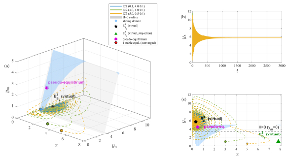
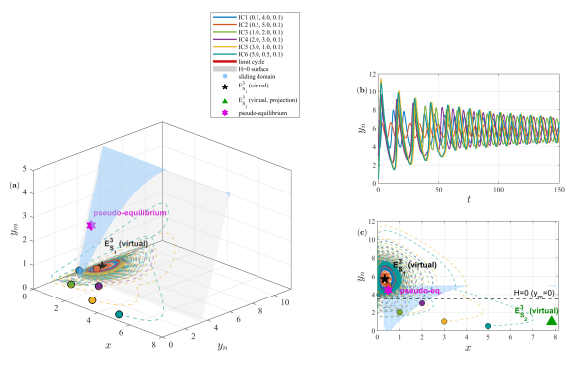
$ (a) $ three-dimensional state-space trajectory plot in $ (x, y_n, y_m) $ space; $ (b) $ time Series plot; $ (c) $ phase projection plot in $ (x, y_n) $ space. Parameters of system (2.1): $ K = 10 $, $ a_n = 0.7 $, $ b = 0.1 $, $ c = 0.5 $, $ \mu_n = 0.18 $, $ \mu_m = 0.18 $, $ \eta_1 = 0.8 $, $ \eta_2 = 0.9 $, $ \alpha = 0.5 $, $ \delta = 0.12 $, $ r = 4 $, $ \gamma = 3.5 $, $ \beta = 0.5 $
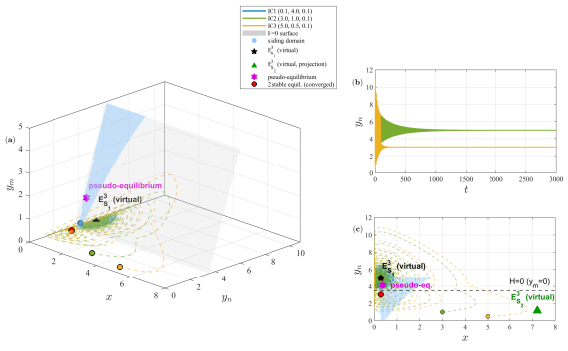
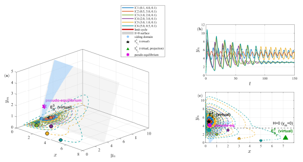
$ (a) $ three-dimensional state-space trajectory plot in $ (x, y_n, y_m) $ space; $ (b) $ time Series plot; $ (c) $ phase projection plot in $ (x, y_n) $ space. Parameters of system (2.1): $ K = 10 $, $ a_n = 0.8 $, $ b = 0.1 $, $ c = 0.5 $, $ \mu_n = 0.18 $, $ \mu_m = 0.18 $, $ \eta_1 = 0.8 $, $ \eta_2 = 0.9 $, $ \alpha = 0.5 $, $ \delta = 0.12 $, $ r = 4 $, $ \gamma = 3.5 $, $ \beta = 0.5 $
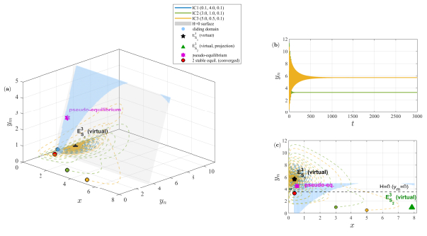
$ (a) $ three-dimensional state-space trajectory plot in $ (x, y_n, y_m) $ space; $ (b) $ time Series plot; $ (c) $ phase projection plot in $ (x, y_n) $ space. Parameters of system (2.1): $ K = 10 $, $ a_n = 0.7 $, $ b = 0.1 $, $ c = 0.5 $, $ \mu_n = 0.20 $, $ \mu_m = 0.18 $, $ \eta_1 = 0.8 $, $ \eta_2 = 0.9 $, $ \alpha = 0.5 $, $ \delta = 0.12 $, $ r = 4 $, $ \gamma = 3.5 $, $ \beta = 0.5 $
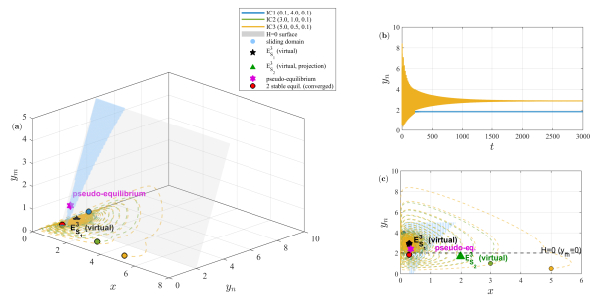
$ (a) $ three-dimensional state-space trajectory plot in $ (x, y_n, y_m) $ space; $ (b) $ time Series plot; $ (c) $ phase projection plot in $ (x, y_n) $ space. Parameters of system (2.1): $ K = 10 $, $ a_n = 0.9 $, $ b = 0.1 $, $ c = 0.5 $, $ \mu_n = 0.20 $, $ \mu_m = 0.18 $, $ \eta_1 = 0.8 $, $ \eta_2 = 0.9 $, $ \alpha = 0.5 $, $ \delta = 0.12 $, $ r = 2.6 $, $ \gamma = 2 $, $ \beta = 0.5 $
$ (a) $ three-dimensional state-space trajectory plot in $ (x, y_n, y_m) $ space; $ (b) $ time Series plot; $ (c) $ phase projection plot in $ (x, y_n) $ space. Parameters of system (2.1): $ K = 10 $, $ a_n = 0.7 $, $ b = 0.1 $, $ c = 0.5 $, $ \mu_n = 0.18 $, $ \mu_m = 0.18 $, $ \eta_1 = 0.8 $, $ \eta_2 = 0.9 $, $ \alpha = 0.5 $, $ \delta = 0.12 $, $ r = 4 $, $ \gamma = 3.5 $, $ \beta = 0.5 $. Simulation time $ T = 150 $
$ (a) $ three-dimensional state-space trajectory plot in $ (x, y_n, y_m) $ space; $ (b) $ time Series plot; $ (c) $ phase projection plot in $ (x, y_n) $ space. Parameters of system (2.1): $ K = 10 $, $ a_n = 0.8 $, $ b = 0.1 $, $ c = 0.5 $, $ \mu_n = 0.18 $, $ \mu_m = 0.18 $, $ \eta_1 = 0.8 $, $ \eta_2 = 0.9 $, $ \alpha = 0.5 $, $ \delta = 0.12 $, $ r = 4 $, $ \gamma = 3.5 $, $ \beta = 0.5 $. Simulation time $ T = 150 $
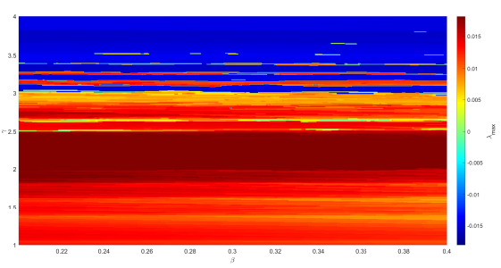
two-dimensional parameter scan of the maximum Lyapunov exponent over the plane $ (\beta, \gamma)\in[0.2, 0.4]\times[1, 4] $ (a uniform $ 200\times 200 $ grid). Parameters of system (2.1): $ K = 10 $, $ a_n = 0.95 $, $ b = 0.1 $, $ c = 0.5 $, $ \mu_n = 0.18 $, $ \mu_m = 0.18 $, $ \eta_1 = 0.8 $, $ \eta_2 = 0.9 $, $ \alpha = 0.5 $, $ \delta = 0.12 $, $ r = 4 $
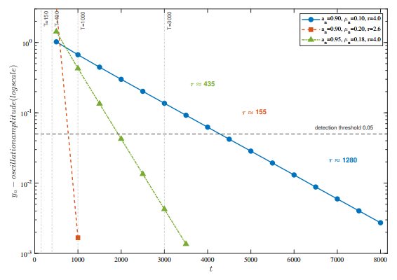
Semi-logarithmic decay curve of oscillation amplitude. The vertical dotted lines mark the stopping instants $ T = 150 $, $ 400 $, $ 1000 $, and $ 3000 $. Parameters of system (2.1): $ \tau = 1280 $: $ K = 10 $, $ a_n = 0.9 $, $ b = 0.1 $, $ c = 0.5 $, $ \mu_n = 0.1 $, $ \mu_m = 0.18 $, $ \eta_1 = 0.8 $, $ \eta_2 = 0.9 $, $ \alpha = 0.5 $, $ \delta = 0.12 $, $ r = 4 $, $ \gamma = 3.5 $, $ \beta = 0.5 $; $ \tau = 155 $: $ K = 10 $, $ a_n = 0.9 $, $ b = 0.1 $, $ c = 0.5 $, $ \mu_n = 0.2 $, $ \mu_m = 0.18 $, $ \eta_1 = 0.8 $, $ \eta_2 = 0.9 $, $ \alpha = 0.5 $, $ \delta = 0.12 $, $ r = 2.6 $, $ \gamma = 3.5 $, $ \beta = 0.5 $; $ \tau = 435 $: $ K = 10 $, $ a_n = 0.95 $, $ b = 0.1 $, $ c = 0.5 $, $ \mu_n = 0.18 $, $ \mu_m = 0.18 $, $ \eta_1 = 0.8 $, $ \eta_2 = 0.9 $, $ \alpha = 0.5 $, $ \delta = 0.12 $, $ r = 4 $, $ \gamma = 3 $, $ \beta = 0.3 $




 DownLoad: