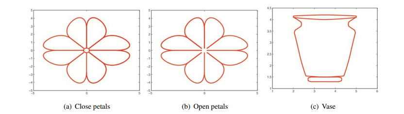
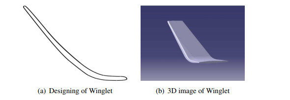
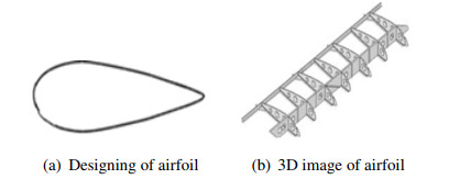
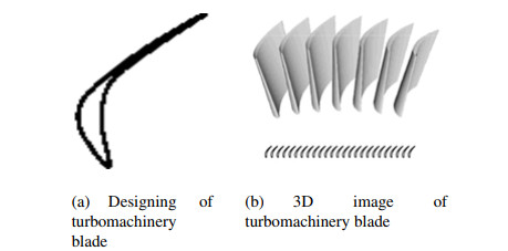
The B-spline curves have been grasped tremendous achievements inside the widely identified field of Computer Aided Geometric Design (CAGD). In CAGD, spline functions have been used for the designing of various objects. In this paper, new Quadratic Trigonometric B-spline (QTBS) functions with two shape parameters are introduced. The proposed QTBS functions inherit the basic properties of classical B-spline and have been proved in this paper. The proposed scheme associated with two shape parameters where the classical B-spline functions do not have. The QTBS has been used for designing of different parts of airplane like winglet, airfoil, turbo-machinery blades and vertical stabilizer. The designed part can be controlled or changed using free parameters. The effect of shape parameters is also expressed.
Citation: Abdul Majeed, Muhammad Abbas, Amna Abdul Sittar, Md Yushalify Misro, Mohsin Kamran. Airplane designing using Quadratic Trigonometric B-spline with shape parameters[J]. AIMS Mathematics, 2021, 6(7): 7669-7683. doi: 10.3934/math.2021445
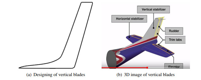
The B-spline curves have been grasped tremendous achievements inside the widely identified field of Computer Aided Geometric Design (CAGD). In CAGD, spline functions have been used for the designing of various objects. In this paper, new Quadratic Trigonometric B-spline (QTBS) functions with two shape parameters are introduced. The proposed QTBS functions inherit the basic properties of classical B-spline and have been proved in this paper. The proposed scheme associated with two shape parameters where the classical B-spline functions do not have. The QTBS has been used for designing of different parts of airplane like winglet, airfoil, turbo-machinery blades and vertical stabilizer. The designed part can be controlled or changed using free parameters. The effect of shape parameters is also expressed.

| [1] | B. Kulfan, J. Bussoletti, Fundamental parameteric geometry representations for aircraft component shapes, 11th AIAA/ISSMO Multidisciplinary Analysis and Optimization Conference, The modeling and simulation frontier for multidisciplinary design optimization, Portsmouth, Virginia, 2006. |
| [2] | J. J. Maisonneuve, D. P. Hills, P. Morelle, C. Fleury, A. J. G. Schoofs, A shape optimisation tool for multi-disciplinary industrial design, In: Computational methods in applied sciences 96: proceedings of the 2nd ECCOMAS conference, Paris, France, 1996,516-522. |
| [3] |
U. Bashir, M. Abbas, M. N. H. Awang, J. M. Ali, A class of quasi-quintic trigonometric Bézier curve with two shape parameters, Science Asia, 39S (2013), 11-15. doi: 10.2306/scienceasia1513-1874.2013.39S.011

|
| [4] | U. Bashir, M. Abbas, J. M. Ali, The G2 and C2 rational quadratic trigonometric Bezier curve with two shape parameters with applications, Appl. Math. Comput., 219 (2013), 10183-10197. |
| [5] |
S. BiBi, M. Abbas, M. Y. Misro, G. Hu, A novel approach of hybrid trigonometric Bézier curve to the modeling of symmetric revolutionary curves and symmetric rotation surfaces, IEEE Access, 7 (2019), 165779-165792. doi: 10.1109/ACCESS.2019.2953496
|
| [6] | S. Maqsood, M. Abbas, G. Hu, A. L. A. Ramli, K. T. Miura, A novel generalization of trigono-metric Bézier curve and surface with shape parameters and its applications, Math. Probl. Eng., 2020 (2020), 4036434. |
| [7] | M. Usman, M. Abbas, K. T. Miura, Some engineering applications of new trigonometric cubic Bézier-like curves to free-form complex curve modeling, J. Adv. Mech. Des. Syst., 14 (2020), 1-15. |
| [8] |
X. Z. Hu, G. Hu, M. Abbas, M. Y. Misro, Approximate multi-degree reduction of Q-Bézier curves via generalized Bernstein polynomial functions, Adv. Differ. Equ., 2020 (2020), 413. doi: 10.1186/s13662-020-02871-y
|
| [9] |
F. H. Li, G. Hu, M. Abbas, K. T. Miura, The generalized H-Bézier model: Geometric continuity conditions and applications to curve and surface modeling, Mathematics, 8 (2020), 924. doi: 10.3390/math8060924
|
| [10] |
A. Majeed, M. Abbas, K. T. Miura, M. Kamran, T. Nazir, Surface modeling from 2D contours with an application to craniofacial fracture construction, Mathematics, 8 (2020), 1246. doi: 10.3390/math8101793
|
| [11] |
G. Hu, H. N. Li, M. Abbas, K. T. Miura, G. L. Wei, Explicit continuity conditions for G1 connection of S-$\lambda $ curves and surfaces, Mathematics, 8 (2020), 1359. doi: 10.3390/math8081359
|
| [12] |
B. M. Kulfan, Universal parametric geometry representation method, J. Aircraft, 45 (2008), 142-158. doi: 10.2514/1.29958
|
| [13] | A. Majeed, A. R. M. Piah, Image reconstruction using rational Ball interpolant and genetic algorithm, Appl. Math. Sci., 8 (2014), 3683-3692. |
| [14] | A. Majeed, A. R. M. Piah, Reconstruction of craniofacial image using rational cubic Ball interpolant and soft computing technique, In: AIP Conference Proceedings, 1682 (2015), 030001. |
| [15] | W. P. Henderson, The effect of canard and vertical tails on the aerodynamic characteristics of a model with a 59 deg sweptback wing at a Mach number of 0.30, 1974. |
| [16] | M. Maughmer, The design of winglets for low-speed aircraft, Technical Soaring, 30 (2016), 6173. |
| [17] | J. M. Grasmeyer, Multidisciplinary design optimization of a strut-braced wing aircraft, Ph.D. dissertation, Virginia Polytechnic Institute and State University, Blacksburg, USA, 1998. |
| [18] | S. Rajendran, Design of Parametric Winglets and Wing tip devices: A conceptual design approach, Ph.D. dissertation, Linkoping University, SE-58183 Linkoping, Sweden, 2012. |
| [19] |
A. Majeed, M. Kamran, M. K. Iqbal, D. Baleanu, Solving time fractional Burgers and Fishers equations using cubic B-spline approximation method, Adv. Differ. Equ., 2020 (2020), 175. doi: 10.1186/s13662-020-02619-8
|
| [20] |
A. Majeed, M. Abbas, F. Qayyum, K. T. Miura, M. Y. Misro, T. Nazir, Geometric modeling using new Cubic trigonometric B-Spline functions with shape parameter, Mathematics, 8 (2020), 2102. doi: 10.3390/math8101793
|
| [21] |
A. Majeed, F. Qayyum, New rational cubic trigonometric B-spline curves with two shape parameters, Comput. Appl. Math., 39 (2020), 1-24. doi: 10.1007/s40314-019-0964-8
|
| [22] |
X. L. Han, Quadratic trigonometric polynomial curves with a shape parameter, Comput. Aided Geom. D., 21 (2004), 535-548. doi: 10.1016/j.cagd.2004.03.001
|
| [23] |
X. L. Han, Piecewise quadratic trigonometric polynomial curves, Math. Comput., 72 (2003), 1369-1377. doi: 10.1090/S0025-5718-03-01530-8
|
| [24] | J. Lin, S. Reutskiy, A cubic B-spline semi-analytical algorithm for simulation of 3D steady-state convection- diffusion-reaction problems. Appl. Math. Comput., 371 (2020), 124944. |
| [25] |
S. Reutskiy, Y. H. Zhang, J. Lin, H. G. Sun, Novel numerical method based on cubic B-splines for a class of nonlinear generalized telegraph equations in irregular domains, Alex. Eng. J., 59 (2020), 77-90. doi: 10.1016/j.aej.2019.12.009
|
| [26] |
S. Reutskiy, J. Lin, B. Zheng, J. Y. Tong, A novel B-Spline method for modeling transport problems in anisotropic inhomogeneous Media, Adv. Appl. Math. Mech., 13 (2021), 590-618. doi: 10.4208/aamm.OA-2020-0052
|
| [27] |
G. Hu, J. L. Wu, X. Q. Qin, A novel extension of the Bezier model and its applications to surface modeling, Adv. Eng. Softw., 125 (2018), 27-54. doi: 10.1016/j.advengsoft.2018.09.002
|
| [28] |
G. Hu, J. L. Wu, Generalized quartic H-Bezier curves: Construction and application to developable surfaces, Adv. Eng. Softw., 138 (2019), 102723. doi: 10.1016/j.advengsoft.2019.102723
|
| [29] | G. Hu, C. C. Bo, G. Wei, X. Q. Qin, Shape-adjustable generalized Bezier surfaces: Construction and it is geometric continuity conditions, Appl. Math. Comput., 378 (2020), 125215. |
Figures(13) / Tables(2)

Abdul Majeed, Muhammad Abbas, Amna Abdul Sittar, Md Yushalify Misro, Mohsin Kamran. Airplane designing using Quadratic Trigonometric B-spline with shape parameters[J]. AIMS Mathematics, 2021, 6(7): 7669-7683. doi: 10.3934/math.2021445


 DownLoad: