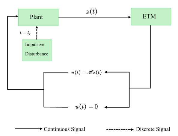
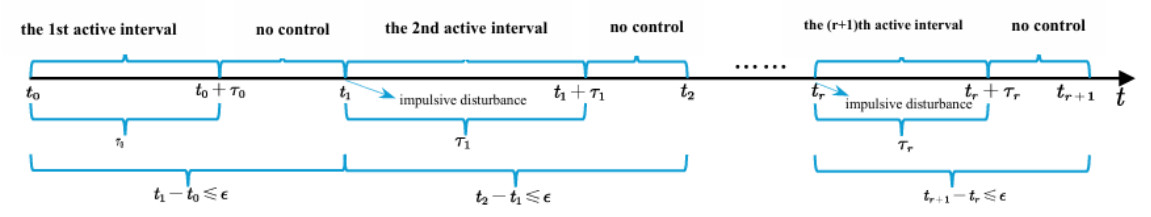
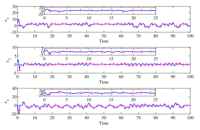
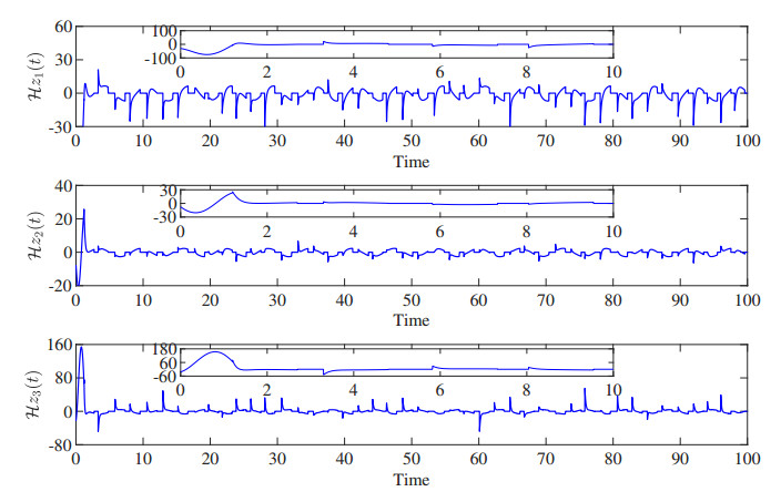
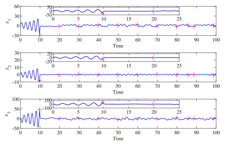
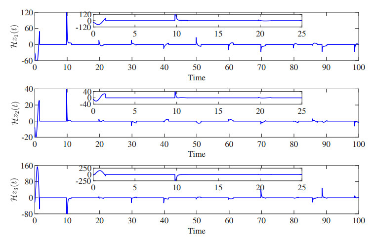
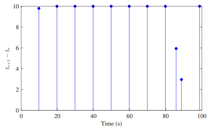
In this paper, the exponential input-to-state stabilization (EISS) problem for nonlinear systems subject to impulsive disturbance and continuous external inputs is addressed by an aperiodic intermittent control (APIC), which is further classified as either time-triggered APIC (TAPIC) or event-triggered APIC (EAPIC). To establish sufficient conditions for the realization of EISS, the Lyapunov approach is used. It is shown that the suggested APIC can successfully reduce the negative consequences of continuous external inputs and impulsive disturbance. Limiting the percentage of the active interval in the control procedure yields a range of impulse moments under TAPIC. The relationship among impulse disturbance, intermittent control parameters, the event-triggered mechanism (ETM), and the threshold is established under EAPIC to guarantee EISS. The predesigned ETM is used to generate a series of impulse disturbance moments. Furthermore, the Zeno phenomenon is excluded. Finally, an example of Chua's oscillator is presented to show how effective the system is under TAPIC and EAPIC.
Citation: Siyue Yao, Jin-E Zhang. Exponential input-to-state stability of nonlinear systems under impulsive disturbance via aperiodic intermittent control[J]. AIMS Mathematics, 2025, 10(5): 10787-10805. doi: 10.3934/math.2025490
In this paper, the exponential input-to-state stabilization (EISS) problem for nonlinear systems subject to impulsive disturbance and continuous external inputs is addressed by an aperiodic intermittent control (APIC), which is further classified as either time-triggered APIC (TAPIC) or event-triggered APIC (EAPIC). To establish sufficient conditions for the realization of EISS, the Lyapunov approach is used. It is shown that the suggested APIC can successfully reduce the negative consequences of continuous external inputs and impulsive disturbance. Limiting the percentage of the active interval in the control procedure yields a range of impulse moments under TAPIC. The relationship among impulse disturbance, intermittent control parameters, the event-triggered mechanism (ETM), and the threshold is established under EAPIC to guarantee EISS. The predesigned ETM is used to generate a series of impulse disturbance moments. Furthermore, the Zeno phenomenon is excluded. Finally, an example of Chua's oscillator is presented to show how effective the system is under TAPIC and EAPIC.

| [1] |
Y. Li, K. W. Wong, X. F. Liao, C. D. Li, On impulsive control for synchronization and its application to the nuclear spin generator system, Nonlinear Anal. Real World Appl., 10 (2009), 1712–1716. https://doi.org/10.1016/j.nonrwa.2008.02.011 doi: 10.1016/j.nonrwa.2008.02.011

|
| [2] | A. Pentari, G. Tzagkarakis, K. Marias, P. Tsakalides, Graph-based denoising of EEG signals in impulsive environments, In: 2020 28th European Signal Processing Conference (EUSIPCO), 2021, 1095–1099. https://doi.org/10.23919/Eusipco47968.2020.9287329 |
| [3] |
X. D. Li, X. Y. Yang, T. W. Huang, Persistence of delayed cooperative models: impulsive control method, Appl. Math. Comput., 342 (2019), 130–146. https://doi.org/10.1016/j.amc.2018.09.003 doi: 10.1016/j.amc.2018.09.003
|
| [4] | Y. Masutani, M. Matsushita, F. Miyazaki, Flyaround maneuvers on a satellite orbit by impulsive thrust control, In: Proceedings 2001 ICRA. IEEE International Conference on Robotics and Automation (Cat. No. 01CH37164), 2001,421–426. https://doi.org/10.1109/ROBOT.2001.932587 |
| [5] |
X. Y. Zhang, C. D. Li, H. F. Li, Finite-time stabilization of nonlinear systems via impulsive control with state-dependent delay, J. Franklin Inst., 359 (2022), 1196–1214. https://doi.org/10.1016/j.jfranklin.2021.11.013 doi: 10.1016/j.jfranklin.2021.11.013
|
| [6] |
Y. C. He, Y. Z. Bai, Finite-time stability and applications of positive switched linear delayed impulsive systems, Math. Model. Control, 4 (2024), 178–194. https://doi.org/10.3934/mmc.2024016 doi: 10.3934/mmc.2024016
|
| [7] |
S. C. Wu, X. D. Li, Finite-time stability of nonlinear systems with delayed impulses, IEEE Trans. Syst. Man Cybern. Syst., 53 (2023), 7453–7460. https://doi.org/10.1109/TSMC.2023.3298071 doi: 10.1109/TSMC.2023.3298071
|
| [8] |
X. Xie, X. D. Li, X. Z. Liu, Event-triggered impulsive control for multi-agent systems with actuation delay and continuous/periodic sampling, Chaos Solitons Fract., 175 (2023), 114067. https://doi.org/10.1016/j.chaos.2023.114067 doi: 10.1016/j.chaos.2023.114067
|
| [9] |
W. J. Sun, M. Z. Wang, J. W. Xia, X. D. Li, Input-to-state stabilization of nonlinear systems with impulsive disturbance via event-triggered impulsive control, Appl. Math. Comput., 497 (2025), 129365. https://doi.org/10.1016/j.amc.2025.129365 doi: 10.1016/j.amc.2025.129365
|
| [10] |
W. L. He, F. Qian, Q. L. Han, G. R. Chen, Almost sure stability of nonlinear systems under random and impulsive sequential attacks, IEEE Trans. Autom. Control, 65 (2020), 3879–3886. https://doi.org/10.1109/TAC.2020.2972220 doi: 10.1109/TAC.2020.2972220
|
| [11] |
J. J. Yang, J. Q. Lu, J. G. Lou, Y. Liu, Synchronization of drive-response Boolean control networks with impulsive disturbances, Appl. Math. Comput., 364 (2020), 124679. https://doi.org/10.1016/j.amc.2019.124679 doi: 10.1016/j.amc.2019.124679
|
| [12] |
X. Y. Yang, X. D. Li, P. Y. Duan, Finite-time lag synchronization for uncertain complex networks involving impulsive disturbances, Neural Comput. Appl., 34 (2022), 5097–5106. https://doi.org/10.1007/s00521-021-05987-8 doi: 10.1007/s00521-021-05987-8
|
| [13] | E. D. Sontag, Smooth stabilization implies coprime factorization, IEEE Trans. Autom. Control, 34 (1989), 435–443. |
| [14] |
P. Li, X. D. Li, J. Q. Lu, Input-to-state stability of impulsive delay systems with multiple impulses, IEEE Trans. Autom. Control, 66 (2021), 362–368. https://doi.org/10.1109/TAC.2020.2982156 doi: 10.1109/TAC.2020.2982156
|
| [15] |
Y. Guo, M. Y. Duan, P. F. Wang, Input-to-state stabilization of semilinear systems via aperiodically intermittent event-triggered control, IEEE Trans. Control Netw. Syst., 9 (2022), 731–741. https://doi.org/10.1109/TCNS.2022.3165511 doi: 10.1109/TCNS.2022.3165511
|
| [16] |
P. L. Yu, F. Q. Deng, X. Y. Zhao, Y. J. Huang, Stability analysis of nonlinear systems in the presence of event-triggered impulsive control, Int. J. Robust Nonlinear Control, 34 (2024), 3835–3853. https://doi.org/10.1002/rnc.7165 doi: 10.1002/rnc.7165
|
| [17] |
X. D. Li, P. Li, Input-to-state stability of nonlinear systems: event-triggered impulsive control, IEEE Trans. Autom. Control, 67 (2022), 1460–1465. https://doi.org/10.1109/TAC.2021.3063227 doi: 10.1109/TAC.2021.3063227
|
| [18] |
F. Shi, Y. Liu, Y. Y. Li, J. L. Qiu, Input-to-state stability of nonlinear systems with hybrid inputs and delayed impulses, Nonlinear Anal. Hybrid Syst., 44 (2022), 101145. https://doi.org/10.1016/j.nahs.2021.101145 doi: 10.1016/j.nahs.2021.101145
|
| [19] |
P. F. Wang, X. L. Wang, H. Su, Input-to-state stability of impulsive stochastic infinite dimensional systems with Poisson jumps, Automatica, 128 (2021), 109553. https://doi.org/10.1016/j.automatica.2021.109553 doi: 10.1016/j.automatica.2021.109553
|
| [20] |
Q. T. Gan, Exponential synchronization of stochastic Cohen-Grossberg neural networks with mixed time-varying delays and reaction-diffusion via periodically intermittent control, Neural Netw., 31 (2012), 12–21. https://doi.org/10.1016/j.neunet.2012.02.039 doi: 10.1016/j.neunet.2012.02.039
|
| [21] |
W. H. Chen, J. C. Zhong, W. X. Zheng, Delay-independent stabilization of a class of time-delay systems via periodically intermittent control, Automatica, 71 (2016), 89–97. https://doi.org/10.1016/j.automatica.2016.04.031 doi: 10.1016/j.automatica.2016.04.031
|
| [22] |
S. J. Yang, C. D. Li, T. W. Huang, Exponential stabilization and synchronization for fuzzy model of memristive neural networks by periodically intermittent control, Neural Netw., 75 (2016), 162–172. https://doi.org/10.1016/j.neunet.2015.12.003 doi: 10.1016/j.neunet.2015.12.003
|
| [23] |
B. Liu, M. Yang, T. Liu, D. J. Hill, Stabilization to exponential input-to-state stability via aperiodic intermittent control, IEEE Trans. Autom. Control, 66 (2021), 2913–2919. https://doi.org/10.1109/TAC.2020.3014637 doi: 10.1109/TAC.2020.3014637
|
| [24] |
M. Liu, H. J. Jiang, C. Hu, Finite-time synchronization of delayed dynamical networks via aperiodically intermittent control, J. Franklin Inst., 354 (2017), 5374–5397. https://doi.org/10.1016/j.jfranklin.2017.05.030 doi: 10.1016/j.jfranklin.2017.05.030
|
| [25] |
X. R. Zhang, Q. Z. Wang, B. Z. Fu, Further stabilization criteria of continuous systems with aperiodic time-triggered intermittent control, Commun. Nonlinear Sci. Numer. Simul., 125 (2023), 107387. https://doi.org/10.1016/j.cnsns.2023.107387 doi: 10.1016/j.cnsns.2023.107387
|
| [26] |
L. Y. You, X. Y. Yang, S. C. Wu, X. D. Li, Finite-time stabilization for uncertain nonlinear systems with impulsive disturbance via aperiodic intermittent control, Appl. Math. Comput., 443 (2023), 127782. https://doi.org/10.1016/j.amc.2022.127782 doi: 10.1016/j.amc.2022.127782
|
| [27] |
Y. Guo, S. Wang, Z. H. Duan, P. F. Wang, Exponential input-to-state stabilization of semilinear systems via intermittent control, Int. J. Robust Nonlinear Control, 33 (2023), 2986–3003. https://doi.org/10.1002/rnc.6548 doi: 10.1002/rnc.6548
|
| [28] |
Y. Zhai, S. Gao, H. Su, Stabilization of delayed nonlinear systems via periodically intermittent event-triggered control, Int. J. Robust Nonlinear Control, 32 (2022), 7843–7859. https://doi.org/10.1002/rnc.6248 doi: 10.1002/rnc.6248
|
| [29] |
W. J. Sun, X. D. Li, Aperiodic intermittent control for exponential input-to-state stabilization of nonlinear impulsive systems, Nonlinear Anal. Hybrid Syst., 50 (2023), 101404. https://doi.org/10.1016/j.nahs.2023.101404 doi: 10.1016/j.nahs.2023.101404
|
| [30] |
D. X. Peng, X. D. Li, R. Rakkiyappan, Y. H. Ding, Stabilization of stochastic delayed systems: event-triggered impulsive control, Appl. Math. Comput., 401 (2021), 126054. https://doi.org/10.1016/j.amc.2021.126054 doi: 10.1016/j.amc.2021.126054
|
| [31] |
M. Z. Wang, X. D. Li, P. Y. Duan, Event-triggered delayed impulsive control for nonlinear systems with application to complex neural networks, Neural Netw., 150 (2022), 213–221. https://doi.org/10.1016/j.neunet.2022.03.007 doi: 10.1016/j.neunet.2022.03.007
|
| [32] |
Y. C. Liu, N. Zhao, Adaptive dynamic event-triggered asymptotic control for uncertain nonlinear systems, Chaos Solitons Fract., 189 (2024), 115597. https://doi.org/10.1016/j.chaos.2024.115597 doi: 10.1016/j.chaos.2024.115597
|
| [33] |
X. D. Liu, F. Q. Deng, W. Wei, F. Z. Wan, P. L. Yu, Periodically intermittent control for stochastic nonlinear delay systems with dynamic event-triggered mechanism, Int. J. Robust Nonlinear Control, 33 (2023), 9665–9683. https://doi.org/10.1002/rnc.6867 doi: 10.1002/rnc.6867
|
| [34] |
Y. N. Wang, C. D. Li, H. J. Wu, H. Deng, Stabilization of nonlinear delayed systems subject to impulsive disturbance via aperiodic intermittent control, J. Franklin Inst., 361 (2024), 106675. https://doi.org/10.1016/j.jfranklin.2024.106675 doi: 10.1016/j.jfranklin.2024.106675
|
| [35] | J. P. Hespanha, A. S. Morse, Stability of switched systems with average dwell-time, In: Proceedings of the 38th IEEE Conference on Decision and Control (Cat. No.99CH36304), 1999, 2655–2660. https://doi.org/10.1109/CDC.1999.831330 |
| [36] |
E. N. Sanchez, J. P. Perez, Input-to-state stability (ISS) analysis for dynamic neural networks, IEEE Trans. Circuits Syst. Ⅰ Fundam. Theory Appl., 46 (1999), 1395–1398. https://doi.org/10.1109/81.802844 doi: 10.1109/81.802844
|
| [37] |
C. D. Li, G. Feng, X. F. Liao, Stabilization of nonlinear systems via periodically intermittent control, IEEE Trans. Circuits Syst. Ⅱ Express Briefs, 54 (2007), 1019–1023. https://doi.org/ 10.1109/TCSII.2007.903205 doi: 10.1109/TCSII.2007.903205
|

Figures(8)

Siyue Yao, Jin-E Zhang. Exponential input-to-state stability of nonlinear systems under impulsive disturbance via aperiodic intermittent control[J]. AIMS Mathematics, 2025, 10(5): 10787-10805. doi: 10.3934/math.2025490


 DownLoad: