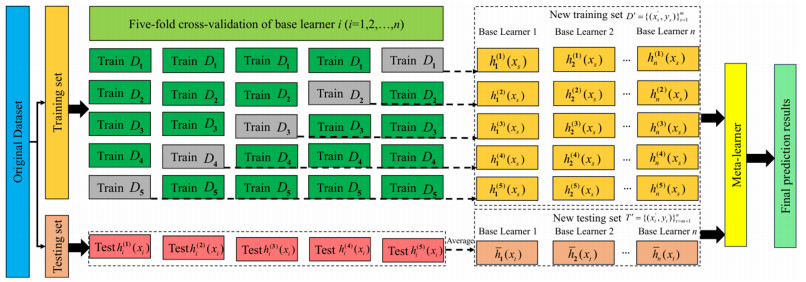
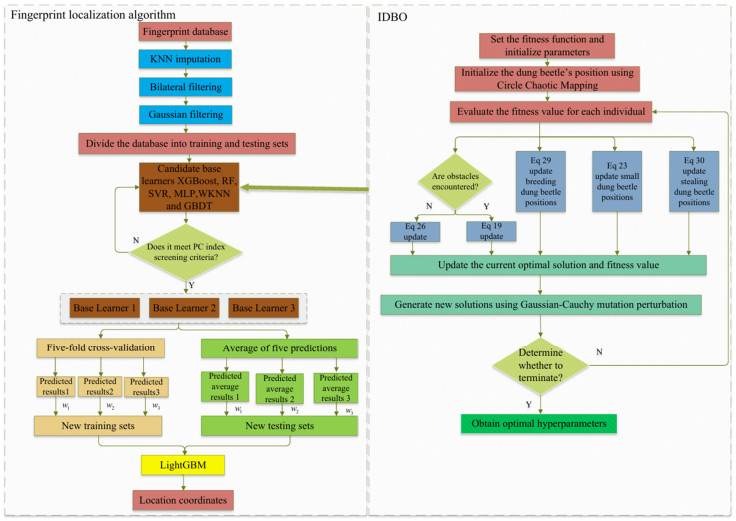
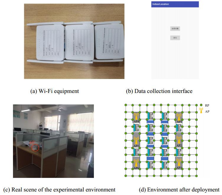
Wi-Fi fingerprint-based indoor localization has garnered significant attention due to its low cost, easy deployment, and high accuracy. However, indoor signal fluctuations and existing method limitations—such as single algorithm usage, low accuracy, and poor generalization—lead to suboptimal localization precision and stability. To address these issues, this paper proposes an improved dung beetle optimizer (IDBO)–stacking indoor fingerprint localization algorithm based on uncertainty estimation. In the offline phase, a hybrid filtering method combining bilateral and Gaussian filtering is first applied to the received signal strength indication (RSSI) fingerprint data for denoising and edge feature preservation, improving the stability of the fingerprint database. Next, the combination of base learners with complementary performance is constructed. An index combining the Pearson coefficient and cosine similarity (the PC index) is designed to select candidate learners with good localization performance and significant diversity as base learners. Meanwhile, IDBO is introduced, which integrates circle chaotic mapping, osprey optimization, variable spiral searching, and Gaussian–Cauchy mutation to perform hyperparameter optimization for the learners. Finally, the training of the base learners and the meta-learner is completed and saved for subsequent online localization. In the online phase, the RSSI signal of the target device is collected in real time and input into the trained base learners. Using the proposed dynamic weight allocation method with uncertainty estimation, the fusion weights of each base learner are dynamically adjusted according to their performance on different data subsets. The final positioning coordinates are output by the meta-learner. Experimental results show that the proposed algorithm achieves an average error of 1.04 m, reducing error by 13.46% to 36.54% compared with other ensemble methods and single algorithms. Moreover, the cumulative distribution function curve converges faster, demonstrating superior positioning performance and strong noise robustness. Moreover, validation in different environments further demonstrates the algorithm's strong adaptability and generalization ability.
Citation: Xinpeng Zheng, Lieping Zhang, Shenglan Zhang, Cui Zhang, Shiyi Xue. IDBO-stacking indoor fingerprint localization algorithm based on uncertainty estimation[J]. Electronic Research Archive, 2025, 33(6): 3756-3793. doi: 10.3934/era.2025167
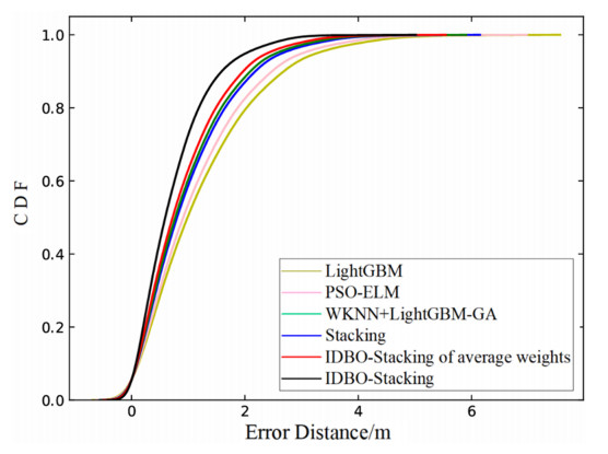
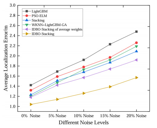
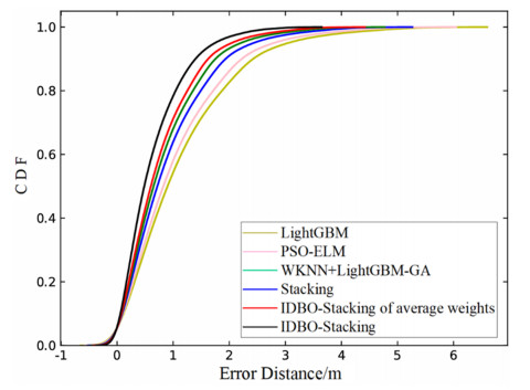
Wi-Fi fingerprint-based indoor localization has garnered significant attention due to its low cost, easy deployment, and high accuracy. However, indoor signal fluctuations and existing method limitations—such as single algorithm usage, low accuracy, and poor generalization—lead to suboptimal localization precision and stability. To address these issues, this paper proposes an improved dung beetle optimizer (IDBO)–stacking indoor fingerprint localization algorithm based on uncertainty estimation. In the offline phase, a hybrid filtering method combining bilateral and Gaussian filtering is first applied to the received signal strength indication (RSSI) fingerprint data for denoising and edge feature preservation, improving the stability of the fingerprint database. Next, the combination of base learners with complementary performance is constructed. An index combining the Pearson coefficient and cosine similarity (the PC index) is designed to select candidate learners with good localization performance and significant diversity as base learners. Meanwhile, IDBO is introduced, which integrates circle chaotic mapping, osprey optimization, variable spiral searching, and Gaussian–Cauchy mutation to perform hyperparameter optimization for the learners. Finally, the training of the base learners and the meta-learner is completed and saved for subsequent online localization. In the online phase, the RSSI signal of the target device is collected in real time and input into the trained base learners. Using the proposed dynamic weight allocation method with uncertainty estimation, the fusion weights of each base learner are dynamically adjusted according to their performance on different data subsets. The final positioning coordinates are output by the meta-learner. Experimental results show that the proposed algorithm achieves an average error of 1.04 m, reducing error by 13.46% to 36.54% compared with other ensemble methods and single algorithms. Moreover, the cumulative distribution function curve converges faster, demonstrating superior positioning performance and strong noise robustness. Moreover, validation in different environments further demonstrates the algorithm's strong adaptability and generalization ability.

| [1] |
S. H. Lee, D. H. Seo, Region clustering based fingerprint model for flexible Wi-Fi fingerprinting, Expert Syst. Appl., 249 (2024), 123389. https://doi.org/10.1016/j.eswa.2024.123389 doi: 10.1016/j.eswa.2024.123389

|
| [2] |
Y. Lin, K. Yu, F. Zhu, J. Bu, X. Dua, The state of the art of deep learning-based Wi-Fi indoor positioning: A review, IEEE Sens. J., 24 (2024), 27076–27098. https://doi.org/10.1109/JSEN.2024.3432154 doi: 10.1109/JSEN.2024.3432154
|
| [3] |
C. Wu, Y. Wang, W. Ke, X. Yang, A dual-branch convolutional neural network-based bluetooth low energy indoor positioning algorithm by fusing received signal strength with angle of arrival, Mathematics, 12 (2024), 2658. https://doi.org/10.3390/math12172658 doi: 10.3390/math12172658
|
| [4] |
J. Guo, Q. Zhao, L. Guo, S. Guo, G. Liang, An improved signal detection algorithm for a mining-purposed MIMO-OFDM IoT-based system, Electron. Res. Arch., 31 (2023), 3943–3962. https://doi.org/10.3934/era.2023200 doi: 10.3934/era.2023200
|
| [5] |
S. Bastiaens, M. Alijani, W. Joseph, D. Plets, Visible light positioning as a next-generation indoor positioning technology: A tutorial, IEEE Commun. Surv. Tutorials, 26 (2024), 2867–2913. https://doi.org/10.1109/COMST.2024.3372153 doi: 10.1109/COMST.2024.3372153
|
| [6] |
L. Wu, S. Guo, L. Han, C. Baris, Indoor positioning method for pedestrian dead reckoning based on multi-source sensors, Measurement, 229 (2024), 114416. https://doi.org/10.1016/j.measurement.2024.114416 doi: 10.1016/j.measurement.2024.114416
|
| [7] |
S. Shang, L. Wang, Overview of WiFi fingerprinting-based indoor positioning, IET Commun., 16 (2022), 725–733. https://doi.org/10.1049/cmu2.1238 doi: 10.1049/cmu2.1238
|
| [8] |
Q. Shen, Y. Cui, WiFi fingerprint correction for indoor localization based on distance metric learning, IEEE Sens. J., 24 (2024), 36167–36177. https://doi.org/10.1109/JSEN.2024.3462759 doi: 10.1109/JSEN.2024.3462759
|
| [9] |
B. Hou, Y. Wang, Positioning by floors based on Wi-Fi fingerprint, Meas. Sci. Technol., 35 (2024), 045003. https://doi.org/10.1088/1361-6501/ad179e doi: 10.1088/1361-6501/ad179e
|
| [10] |
S. Wan, C. Gu, Y. Shu, Z. Shi, Last-seen time is critical: revisiting RSSI-based Wi-Fi indoor localization, Signal Process., 231 (2025), 109756. https://doi.org/10.1016/j.sigpro.2024.109756 doi: 10.1016/j.sigpro.2024.109756
|
| [11] |
M. Mallik, A. K. Panja, C. Chowdhury, Paving the way with machine learning for seamless indoor-outdoor positioning: A survey, Inf. Fusion, 94 (2023), 126–151. https://doi.org/10.1016/j.inffus.2023.01.023 doi: 10.1016/j.inffus.2023.01.023
|
| [12] |
D. J. Suroso, F. Y. M. Adiyatma, C-MEL: Consensus-based multiple ensemble learning for indoor device-free localization through fingerprinting, IEEE Access, 12 (2024), 166381–166392. https://doi.org/10.1109/ACCESS.2024.3493889 doi: 10.1109/ACCESS.2024.3493889
|
| [13] |
J. Wisanmongkol, A. Taparugssanagorn, L. C. Tran, T. L. Anh, X. J. Huang, R. Christian, et al., An ensemble approach to deep-learning-based wireless indoor localization, IET Wireless Sens. Syst., 12 (2022), 33–55. https://doi.org/10.1049/wss2.12035 doi: 10.1049/wss2.12035
|
| [14] |
A. Mohammed, R. Kora, A comprehensive review on ensemble deep learning: Opportunities and challenges, J. King Saud Univ. Comput. Inf. Sci., 35 (2023), 757–774. https://doi.org/10.1016/j.jksuci.2023.01.014 doi: 10.1016/j.jksuci.2023.01.014
|
| [15] |
J. H. Park, D. Kim, Y. J. Suh, WKNN-based Wi-Fi fingerprinting with deep distance metric learning via siamese triplet network for indoor positioning, Electronics, 13 (2024), 4448. https://doi.org/10.3390/electronics13224448 doi: 10.3390/electronics13224448
|
| [16] |
L. Yin, P. Ma, Z. Deng, JLGBMLoc—A novel high-precision indoor localization method based on lightgbM, Sensors, 21 (2021), 2722. https://doi.org/10.3390/s21082722 doi: 10.3390/s21082722
|
| [17] |
D. Gufran, S. Tiku, S. Pasricha, SANGRIA: Stacked autoencoder neural networks with gradient boosting for indoor localization, IEEE Embedded Syst. Lett., 16 (2024), 142–145. https://doi.org/10.1109/LES.2023.3279017 doi: 10.1109/LES.2023.3279017
|
| [18] |
Q. Wanqing, Z. Qingmiao, Z. Junhui, Y. Lihua, Improved PSO-extreme learning machine algorithm for indoor localization, China Commun., 21 (2024), 113–122. https://doi.org/10.23919/JCC.fa.2022-0011.202405 doi: 10.23919/JCC.fa.2022-0011.202405
|
| [19] |
J. Bi, M. Zhao, G. Yao, H. Cao, Y. Feng, H. Jiang, et al., PSOSVRPos: Wi-Fi indoor positioning using SVR optimized by PSO, Expert Syst. Appl., 222 (2023), 119778. https://doi.org/10.1016/j.eswa.2023.119778 doi: 10.1016/j.eswa.2023.119778
|
| [20] |
B. Chen, J. Ma, L. Zhang, Z. Xiong, J. Fan, H. Lan, An improved weighted KNN fingerprint positioning algorithm, Wireless Netw., 30 (2024), 6011–6022. https://doi.org/10.1007/s11276-023-03400-x doi: 10.1007/s11276-023-03400-x
|
| [21] |
Y. Wang, C. Xue, Y. Xia, S. Sun, M. Liu, RF-CPO-SVR algorithm for indoor localization based on Wi-Fi fingerprints, Meas. Sci. Technol., 36 (2025), 036309. https://doi.org/10.1088/1361-6501/adb200 doi: 10.1088/1361-6501/adb200
|
| [22] |
A. Alitaleshi, H. Jazayeriy, J. Kazemitabar, EA-CNN: A smart indoor 3D positioning scheme based on Wi-Fi fingerprinting and deep learning, Eng. Appl. Artif. Intell., 117 (2023), 105509. https://doi.org/10.1016/j.engappai.2022.105509 doi: 10.1016/j.engappai.2022.105509
|
| [23] |
H. Lu, L. Zhang, H. Chen, S. Zhang, S. Wang, H. Peng, et al., An indoor fingerprint positioning algorithm based on WKNN and improved XGBoost, Sensors, 23 (2023), 3952. https://doi.org/10.3390/s23083952 doi: 10.3390/s23083952
|
| [24] |
N. Liu, Z. Liu, J. Gao, Y. Yuan, K. Chan, Wi-Fi fingerprint-based indoor location: Multiple fingerprints and multiple classifiers with two-layer fusion weights, Int. J. Commun. Syst., 37 (2024), e5828. https://doi.org/10.1002/dac.5828 doi: 10.1002/dac.5828
|
| [25] |
M. Chen, Q. Pu, Bayesian optimized indoor positioning algorithm based on dual clustering, Sci. Rep., 15 (2025), 9272. https://doi.org/10.1038/s41598-024-79647-x doi: 10.1038/s41598-024-79647-x
|
| [26] |
X. Lu, K. Zhong, Z. Guan, J. Liu, A fingerprint location framework for uneven Wi-Fi signals based on machine learning, IEEE Lat. Am. Trans., 22 (2024), 321–328. https://doi.org/10.1109/TLA.2024.10473000 doi: 10.1109/TLA.2024.10473000
|
| [27] |
L. Zhang, Y. Chen, X. Gao, X. Zheng, C. Zhang, An algorithm for indoor positioning based on LightGBM+ ExtraTrees chaotic weighted ensemble: evaluation and comparison, J. Supercomput., 81 (2025), 812. https://doi.org/10.1007/s11227-025-07291-x doi: 10.1007/s11227-025-07291-x
|
| [28] |
E. Alalwany, B. Alsharif, Y. Alotaibi, I. Mahgoub, A. Alfahaid, M. Ilyas, Stacking ensemble deep learning for real-time intrusion detection in IoMT environments, Sensors, 25 (2025), 624. https://doi.org/10.3390/s25030624 doi: 10.3390/s25030624
|
| [29] |
J. Q. Wang, Y. J. Wang, G. W. Liu, G. F. Chen, A model stacking algorithm for indoor positioning system using WiFi fingerprinting, KSⅡ Trans. Internet Inf. Syst., 17 (2023), 1200–1215. https://doi.org/10.3837/tiis.2023.04.009 doi: 10.3837/tiis.2023.04.009
|
| [30] |
J. Zhang, X. Yang, W. Zhu, D. Wu, J. Wan, N. Xia, A combined model WAPI indoor localization method based on UMAP, Int. J. Commun. Syst., 38 (2025), e70034. https://doi.org/10.1002/dac.70034 doi: 10.1002/dac.70034
|
| [31] |
Y. Leng, F. Huang, W. Tan, A Wi-Fi fingerprint positioning method based on RLWKNN, IEEE Sens. J., 25 (2024), 1706–1715. https://doi.org/10.1109/JSEN.2024.3476335 doi: 10.1109/JSEN.2024.3476335
|
| [32] |
S. Shafieian, M. Zulkernine, Multi-layer stacking ensemble learners for low footprint network intrusion detection, Complex Intell. Syst., 9 (2023), 3787–3799. https://doi.org/10.1007/s40747-022-00809-3 doi: 10.1007/s40747-022-00809-3
|
| [33] | Y. Dong, H. Zhang, C. Wang, X. Zhou, Wind power forecasting based on stacking ensemble model, decomposition and intelligent optimization algorithm, Neurocomputing, 462 (2021), 169–184. https://doi.org/10.1016/j.neucom.2021.07.084 |
| [34] |
H. Hou, C. Liu, R. Wei, H. He, L. Wang, W. Li, Outage duration prediction under typhoon disaster with stacking ensemble learning, Reliab. Eng. Syst. Saf., 237 (2023), 109398. https://doi.org/10.1016/j.ress.2023.109398 doi: 10.1016/j.ress.2023.109398
|
| [35] |
T. Xia, D. Han, Y. Jiang, Y. Shao, D. Wang, E. Pan, et al., Remaining useful life estimation based on selective ensemble of deep neural networks with diversity, Adv. Eng. Inf., 62 (2024), 102608. https://doi.org/10.1016/j.aei.2024.102608 doi: 10.1016/j.aei.2024.102608
|
| [36] |
C. Zhang, J. Deng, W. Yi, Data-driven online tracking filter architecture: A LightGBM implementation, Signal Process., 221 (2024), 109477. https://doi.org/10.1016/j.sigpro.2024.109477 doi: 10.1016/j.sigpro.2024.109477
|
| [37] |
V. H. Truong, S. Tangaramvong, G. Papazafeiropoulos, An efficient LightGBM-based differential evolution method for nonlinear inelastic truss optimization, Expert Syst. Appl., 237 (2024), 121530. https://doi.org/10.1016/j.eswa.2023.121530 doi: 10.1016/j.eswa.2023.121530
|
| [38] |
H. E. Gorjan, V. P. G Jiménez, Improving indoor Wi-Fi localization by using machine learning techniques, Sensors, 24 (2024), 6293. https://doi.org/10.3390/s24196293 doi: 10.3390/s24196293
|
| [39] | S. Demir, E. K. Sahin, Predicting occurrence of liquefaction-induced lateral spreading using gradient boosting algorithms integrated with particle swarm optimization: PSO-XGBoost, PSO-LightGBM, and PSO-CatBoost, Acta Geotech., 18 (2023), 3403–3419. https://doi.org/10.1007/s11440-022-01777-1 |
| [40] |
L. Yang, A. Shami, On hyperparameter optimization of machine learning algorithms: Theory and practice, Neurocomputing, 415 (2020), 295–316. https://doi.org/10.1016/j.neucom.2020.07.061 doi: 10.1016/j.neucom.2020.07.061
|
| [41] |
B. Bischl, M. Binder, M. Lang, T. Pielok, J. Richter, S. Coors, et al., Hyperparameter optimization: Foundations, algorithms, best practices, and open challenges, Wiley Interdiscip. Rev.: Data Min. Knowl. Discovery, 13 (2023), e1484. https://doi.org/10.1002/widm.1484 doi: 10.1002/widm.1484
|
| [42] |
M. Tayebi, E. S. Kafhali, Performance analysis of metaheuristics based hyperparameters optimization for fraud transactions detection, Evol. Intell., 17 (2024), 921–939. https://doi.org/10.1007/s12065-022-00764-5 doi: 10.1007/s12065-022-00764-5
|
| [43] |
A. Morales-Hernández, I. V Nieuwenhuyse, R. S. Gonzalez, A survey on multi-objective hyperparameter optimization algorithms for machine learning, Artif. Intell. Rev., 56 (2023), 8043–8093. https://doi.org/10.1007/s10462-022-10359-2 doi: 10.1007/s10462-022-10359-2
|
| [44] |
T. Liu, L. Yang, Y. Li, X. Qin, An improved dung beetle optimizer based on Padé approximation strategy for global optimization and feature selection, Electron. Res. Arch., 33 (2025), 1693–1762. https://doi.org/10.3934/era.2025079 doi: 10.3934/era.2025079
|
| [45] |
M. Dehghani, P. Trojovský, Osprey optimization algorithm: A new bio-inspired metaheuristic algorithm for solving engineering optimization problems, Front. Mech. Eng., 8 (2023), 1126450. https://doi.org/10.3389/fmech.2022.1126450 doi: 10.3389/fmech.2022.1126450
|
| [46] |
D. G. Zhang, H. Z. An, J. Zhang, T. Zhang, W. M. Dong, X. R. Jiang, Novel privacy awareness task offloading approach based on privacy entropy, IEEE Trans. Netw. Serv. Manage., 21 (2024), 3598–3608. https://doi.org/10.1109/TNSM.2024.3355967 doi: 10.1109/TNSM.2024.3355967
|
| [47] |
H. Huang, Z. Yao, X. Wei, Y. Zhou, Twin support vector machines based on chaotic mapping dung beetle optimization algorithm, J. Comput. Des. Eng., 11 (2024), 101–110. https://doi.org/10.1093/jcde/qwae040 doi: 10.1093/jcde/qwae040
|
| [48] |
J. Xue, B. Shen, Dung beetle optimizer: A new meta-heuristic algorithm for global optimization, J. Supercomput., 79 (2023), 7305–7336. https://doi.org/10.1007/s11227-022-04959-6 doi: 10.1007/s11227-022-04959-6
|
| [49] |
S. Feng, Y. Hu, D. Hu, Y. Li, R. Hu, Intelligent classification of rocks in mountain highway tunnels using ISSA-ELM model, Geotech. Geol. Eng., 42 (2024), 7385–7405. https://doi.org/10.1007/s10706-024-02931-0 doi: 10.1007/s10706-024-02931-0
|
| [50] | J. Wang, W. Wang, X. Hu, H. Zang, Black-winged kite algorithm: a nature-inspired meta-heuristic for solving benchmark functions and engineering problems. Artif. Intell. Rev., 57 (2024), 98. https://doi.org/10.1007/s10462-024-10723-4 |
| [51] |
R. Storn, K. Price, Differential evolution–a simple and efficient heuristic for global optimization over continuous spaces, J. Global Optim., 11 (1997), 341–359. https://doi.org/10.1023/A:1008202821328 doi: 10.1023/A:1008202821328
|
| [52] |
X. Yang, G. Zhou, Z. Ren, Y. Qiao, J. Yi, High-precision air conditioning load forecasting model based on improved sparrow search algorithm, J. Build. Eng., 92 (2024), 109809. https://doi.org/10.1016/j.jobe.2024.109809 doi: 10.1016/j.jobe.2024.109809
|
| [53] |
M. Shi, L. Deng, B. Yang, L. Qin, L. Gu, Research on internal leakage detection of the ball valves based on stacking ensemble learning, Meas. Sci. Technol., 35 (2024), 095109. https://doi.org/10.1088/1361-6501/ad56b0 doi: 10.1088/1361-6501/ad56b0
|
| [54] |
L. Zhang, X. Zheng, Y. Chen, H. Lu, C. Zhang, Indoor fingerprint localization algorithm based on WKNN and LightGBM-GA, Meas. Sci. Technol., 35 (2024), 116313. https://doi.org/10.1088/1361-6501/ad71eb doi: 10.1088/1361-6501/ad71eb
|
Figures(13) / Tables(9)
Xinpeng Zheng, Lieping Zhang, Shenglan Zhang, Cui Zhang, Shiyi Xue. IDBO-stacking indoor fingerprint localization algorithm based on uncertainty estimation[J]. Electronic Research Archive, 2025, 33(6): 3756-3793. doi: 10.3934/era.2025167


 DownLoad: