Generalized estimation equations method for fixed effects panel interval-valued data models

Chi Liu; Ruiqin Tian; Dengke Xu; Chi Liu; Ruiqin Tian; Dengke Xu

doi:10.3934/era.2025166

Electronic Research Archive

2025, Volume 33, Issue 6: 3733-3755. doi: 10.3934/era.2025166

Previous Article Next Article

Research article

Generalized estimation equations method for fixed effects panel interval-valued data models

1.
School of Mathematics, Hangzhou Normal University, Hangzhou 311121, China
2.
School of Economics, Hangzhou Dianzi University, Hangzhou 310018, China

Received: 24 March 2025 Revised: 13 May 2025 Accepted: 29 May 2025 Published: 16 June 2025

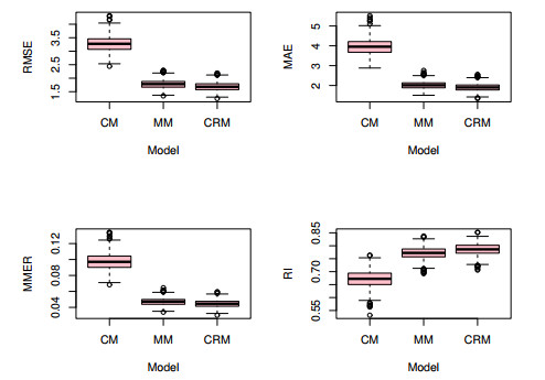
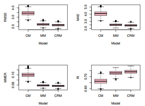
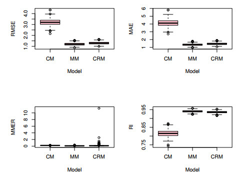
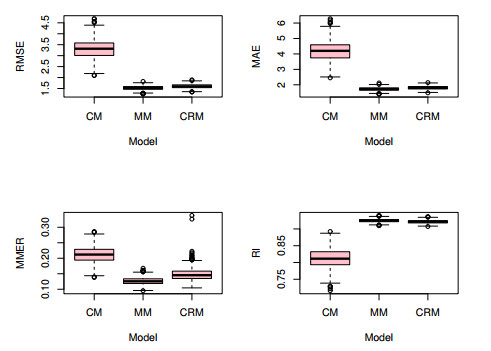
This paper studied panel interval-valued data models with individual fixed effects, in which the correlation within a group was considered and the group average method was used to eliminate the fixed effects. Then, we applied generalized estimation equations (GEEs) to analyze panel interval-valued data models and gave a computational algorithm to obtain the estimators. Some Monte Carlo simulations and real data analysis showed that, in contrast with the least-squares dummy-variable (LSDV) method, the proposed GEEs method has advantages in forecasting performance.
- panel interval-valued data,
- generalized estimation equations,
- the min-max model,
- the center and range model,
- fixed effects
Citation: Chi Liu, Ruiqin Tian, Dengke Xu. Generalized estimation equations method for fixed effects panel interval-valued data models[J]. Electronic Research Archive, 2025, 33(6): 3733-3755. doi: 10.3934/era.2025166

Related Papers:

Abstract

This paper studied panel interval-valued data models with individual fixed effects, in which the correlation within a group was considered and the group average method was used to eliminate the fixed effects. Then, we applied generalized estimation equations (GEEs) to analyze panel interval-valued data models and gave a computational algorithm to obtain the estimators. Some Monte Carlo simulations and real data analysis showed that, in contrast with the least-squares dummy-variable (LSDV) method, the proposed GEEs method has advantages in forecasting performance.

References

[1]	E. Diday, The symbolic approach in clustering and related methods of data analysis, classification and related methods of data analysis, in Proceedings of the first Conference of the Federation of the classification societies. North Holland, 1988.
[2]	L. Billard, E. Diday, Regression analysis for interval-valued data, in Data Analysis, Classification, and Related Methods, Springer, (2000), 369–374.
[3]	L. Billard, E. Diday, Symbolic regression analysis, in Classification, Clustering, and Data Analysis: Recent Advances and Applications, Springer, (2002), 281–288.
[4]	E. d. A. L. Neto, F. D. A. De Carvalho, Centre and range method for fitting a linear regression model to symbolic interval data, Comput. Stat. Data Anal., 52 (2008), 1500–1515. https://doi.org/10.1016/j.csda.2007.04.014 doi: 10.1016/j.csda.2007.04.014
[5]	L. Kong, X. Gao, A regularized MM estimate for interval-valued regression, Expert Syst. Appl., 238 (2024), 122044. https://doi.org/10.1016/j.eswa.2023.122044 doi: 10.1016/j.eswa.2023.122044
[6]	M. Xu, Z. Qin, A bivariate bayesian method for interval-valued regression models, Knowl.-Based Syst., 235 (2022), 107396. https://doi.org/10.1016/j.knosys.2021.107396 doi: 10.1016/j.knosys.2021.107396
[7]	U. Beyaztas, H. L. Shang, A. S. G. Abdel-Salam, Functional linear models for interval-valued data, Commun. Stat.-Simul. Comput., 51 (2022), 3513–3532. https://doi.org/10.1080/03610918.2020.1714662 doi: 10.1080/03610918.2020.1714662
[8]	Q. Zhao, H. Wang, S. Wang, Robust regression for interval-valued data based on midpoints and log-ranges, Adv. Data Anal. Classif., 17 (2023), 583–621. https://doi.org/10.1007/s11634-022-00518-2 doi: 10.1007/s11634-022-00518-2
[9]	L. C. Lin, H. L. Chien, S. Lee, Symbolic interval-valued data analysis for time series based on auto-interval-regressive models, Stat. Method. Appl., 30 (2021), 295–315. https://doi.org/10.1007/s10260-020-00525-7 doi: 10.1007/s10260-020-00525-7
[10]	J. Zhang, M. Liu, M. Dong, Variational bayesian inference for interval regression with an asymmetric laplace distribution, Neurocomputing, 323 (2019), 214–230. https://doi.org/10.1016/j.neucom.2018.09.083 doi: 10.1016/j.neucom.2018.09.083
[11]	C. Yang, Interval riccati equation-based and non-probabilistic dynamic reliability-constrained multi-objective optimal vibration control with multi-source uncertainties, J. Sound Vibr., 595 (2025), 118742. https://doi.org/10.1016/j.jsv.2024.118742 doi: 10.1016/j.jsv.2024.118742
[12]	C. Yang, Y. Liu, H. Gao, Reliability-constrained uncertain spacecraft sliding mode attitude tracking control with interval parameters, IEEE Trans. Aerosp. Electron. Syst., 61 (2025), 1–14. https://doi.org/10.1109/TAES.2025.3529798 doi: 10.1109/TAES.2025.3529798
[13]	A. F. Galvao Jr, Quantile regression for dynamic panel data with fixed effects, J. Econom., 164 (2011), 142–157. https://doi.org/10.1016/j.jeconom.2011.02.016 doi: 10.1016/j.jeconom.2011.02.016
[14]	E. Aristodemou, Semiparametric identification in panel data discrete response models, J. Econom., 220 (2021), 253–271. https://doi.org/10.1016/j.jeconom.2020.04.002 doi: 10.1016/j.jeconom.2020.04.002
[15]	B. H. Beyaztas, S. Bandyopadhyay, Robust estimation for linear panel data models, Stat. Med., 39 (2020), 4421–4438. https://doi.org/10.1002/sim.8732 doi: 10.1002/sim.8732
[16]	J. Bai, S. H. Choi, Y. Liao, Feasible generalized least squares for panel data with cross-sectional and serial correlations, Empir. Econ., 60 (2021), 309–326. https://doi.org/10.1007/s00181-020-01977-2 doi: 10.1007/s00181-020-01977-2
[17]	B. H. Baltagi, D. Li, Prediction in the panel data model with spatial correlation, in Advances in Spatial Econometrics: Methodology, Tools and Applications, Springer, (2004), 283–295.
[18]	J. P. Elhorst, Spatial panel data models, in Spatial Econometrics: From Cross-Sectional Data to Spatial Panels, Springer, (2014), 37–93.
[19]	Y. Zhang, J. Jiang, Y. Feng, Penalized quantile regression for spatial panel data with fixed effects, Commun. Stat.-Theory Methods, 52 (2023), 1287–1299. https://doi.org/10.1080/03610926.2021.1934028 doi: 10.1080/03610926.2021.1934028
[20]	A. Ji, J. Zhang, X. He, Y. Zhang, Fixed effects panel interval-valued data models and applications, Knowl.-Based Syst., 237 (2022), 107798. https://doi.org/10.1016/j.knosys.2021.107798 doi: 10.1016/j.knosys.2021.107798
[21]	J. Zhang, Q. Li, B. Wei, A. Ji, Robust estimation method for panel interval-valued data model with fixed effects, J. Stat. Comput. Simul., 94 (2024), 3230–3251. https://doi.org/10.1080/00949655.2024.2381491 doi: 10.1080/00949655.2024.2381491
[22]	A. Ji, J. Zhang, Y. Cao, Bivariate maximum likelihood method for fixed effects panel interval-valued data models, Comput. Econ., 64 (2024), 1–28. https://doi.org/10.1007/s10614-024-10737-8 doi: 10.1007/s10614-024-10737-8
[23]	K. Y. Liang, S. L. Zeger, Longitudinal data analysis using generalized linear models, Biometrika, 73 (1986), 13–22. https://doi.org/10.1093/biomet/73.1.13 doi: 10.1093/biomet/73.1.13
[24]	M. Crowder, On consistency and inconsistency of estimating equations, Econom. Theory, 2 (1986), 305–330. https://doi.org/10.1017/S0266466600011646 doi: 10.1017/S0266466600011646
[25]	R. M. Balan, I. S. Kratina, Asymptotic results with generalized estimating equations for longitudinal data, Ann. Stat., 33 (2005), 522–541. https://doi.org/10.1214/009053604000001255 doi: 10.1214/009053604000001255
[26]	L. Wang, Gee analysis of clustered binary data with diverging number of covariates, Ann. Stat., 39 (2011), 389–417. https://doi.org/10.1214/10-AOS846 doi: 10.1214/10-AOS846
[27]	Y. G. Wang, V. Carey, Working correlation structure misspecification, estimation and covariate design: implications for generalised estimating equations performance, Biometrika, 90 (2003), 29–41. https://doi.org/10.1093/biomet/90.1.29 doi: 10.1093/biomet/90.1.29
[28]	W. Pan, Model selection in estimating equations, Biometrics, 57 (2001), 529–534. https://doi.org/10.1111/j.0006-341X.2001.00529.x doi: 10.1111/j.0006-341X.2001.00529.x
[29]	M. Wang, Generalized estimating equations in longitudinal data analysis: a review and recent developments, Adv. Stat., 2014 (2014), 303728. https://doi.org/10.1155/2014/303728 doi: 10.1155/2014/303728
[30]	S. Seaman, A. Copas, Doubly robust generalized estimating equations for longitudinal data, Stat. Med., 28 (2009), 937–955. https://doi.org/10.1002/sim.3520 doi: 10.1002/sim.3520
[31]	N. R. Chaganty, An alternative approach to the analysis of longitudinal data via generalized estimating equations, J. Stat. Plan. Infer., 63 (1997), 39–54. https://doi.org/10.1016/S0378-3758(96)00203-0} doi: 10.1016/S0378-3758(96)00203-0
[32]	N. R. Chaganty, J. Shults, On eliminating the asymptotic bias in the quasi-least squares estimate of the correlation parameter, J. Stat. Plan. Infer., 76 (1999), 145–161. https://doi.org/10.1016/S0378-3758(98)00180-3 doi: 10.1016/S0378-3758(98)00180-3
[33]	C. Hu, L. T. He, An application of interval methods to stock market forecasting, Reliab. Comput., 13 (2007), 423–434. https://doi.org/10.1007/s11155-007-9039-4 doi: 10.1007/s11155-007-9039-4

Reader Comments

Your name:*

Email:*
© 2025 the Author(s), licensee AIMS Press. This is an open access article distributed under the terms of the Creative Commons Attribution License (http://creativecommons.org/licenses/by/4.0)