Estimation of partially linear single-index spatial autoregressive model using B-splines

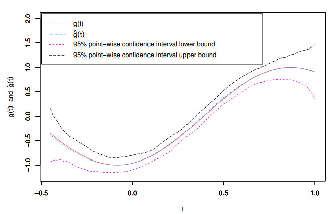
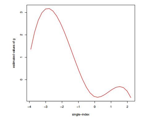
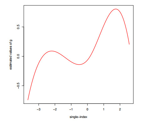
1.   Introduction

In empirical practice of economics and statistics, possible dependence across spatial units is a relevant issue in urban, real estate, regional, public, agricultural, environmental economics, and industrial organization ^[1]. Many studies have proposed approaches and techniques to deal with these problems by imposing some structures on the model in order to capture spatial dependence or spatial autocorrelation in cross-sectional and/or panel data. In recent years, spatial autoregressive (SAR) models have attracted great interest due to their usefulness in practice. For instance, SAR models have the property of using autocorrelation structures according to spatial patterns on data. These models allow for the analysis of spatial dependencies and interactions among observations, making them particularly useful in fields such as geography, environmental science, and urban planning where spatial relationships play crucial roles.

Lee ^[2] explained that ordinary least squares (OLS) estimators can be inconsistent for estimating an SAR model due to the fact that the spatial lagged variables can be correlated with the disturbances in a spatial model. In order to obtain a consistent estimator, Lee ^[1] proposed the quasi-maximum likelihood estimator (QMLE) for the SAR model, investigated the asymptotic properties of QMLE, and found out that the rates of convergence of QMLE may depend on some general features of the spatial weight matrix of the model. However, the quasi-maximum likelihood procedures often pose computational challenges when dealing with large sample sizes, as analytical solutions are not available and numerical methods must be employed to obtain numerical solutions. Kelejian and Prucha ^[3] proposed the generalized spatial two-stage least squares procedure for estimating the SAR model in which they demonstrated consistency and asymptotic normality of the resulting estimator. However, the estimator is not asymptotically effective. Lee ^[4] proposed best spatial two stage least squares estimators for the SAR model to improve the efficiency of the estimator. Su ^[5] extended the SAR to a semi-parametric setting and proposed the GMM estimation method, and showed that the resulting estimator is consistent and asymptotically normal. Xu and Lee ^[6] proposed the maximum likelihood estimator (MLE) for the SAR Tobit model and studied the asymptotic properties.

Recently, there has been a growing literature on semiparametric spatial autoregressive models. Invoking the flexibility of partial linear model, Su and Jin ^[7] developed asymptotic theories for the QMLE of partial linear SAR models based on the profile quasi-maximum likelihood theme. In Su and Jin ^[7], the rate of convergence of the spatial parameter estimator depends on some general features of the spatial weight matrix of the model. Du et al. ^[8] proposed the partial linear additive SAR model. Obviously, the model proposed by Du et al. ^[8] did not impose any interaction within nonparametric components in spatial data. Therefore, the proposed method by Du et al. ^[8] cannot solve the problem of interaction effects on response variables in spatial data. Moreover, the nonparametric components are subject to the curse of dimensionality and can only accommodate low-dimensional covariates; see Wang ^[9]. The single-index model is an important tool in multivariate nonparametric regression. By reducing the dimensionality from multivariate predictors to a univariate index, single-index models avoid the so-called "curse of dimensionality" while still capturing important features in high-dimensional data. Cheng and Chen ^[10] introduced the partially linear single-index spatial autoregressive model (PLSISARM), employing local linear approximation to estimate unknown link functions and utilizing MLE. In contrast to the partial linear SAR model and the partial linear additive SAR model, PLSISARM considers covariate interactions within its nonparametric component. This paper proposes a new estimation procedure for PLSISARM. Specifically, we utilize B-splines to approximate the unknown link function, enhancing smoothness, and adopt QMLE as the estimation method. We also introduce a feasible Nelder-Mead iteration algorithm tailored for this new estimation procedure. Furthermore, we establish the asymptotic properties for the QMLE. Finally, we demonstrate the application of PLSISARM on two distinct datasets from meteorology and economics, thereby extending the practical utility of the model. Compared to Cheng and Chen's work ^[10], B-spline approximation is computationally more efficient and smoother than local linear approximation, facilitating easier interpretation in practical applications. Additionally, this paper employs QMLE instead of MLE, resulting in differences in asymptotic distributions. Notably, when the error term does not satisfy the normal distribution, QMLE can still estimate the asymptotic variance, while MLE fails to do so.

This paper is organized as follows. In Section 2, we describe the technical setting and propose the estimation procedure for PLSISARM via QMLE. In Section 3, we establish the asymptotic properties for the proposed procedure. In Section 4, we present the simulation studies to assess the finite sample performance of the proposed procedure. In Section 5, we analyze two real data sets to illustrate the practical usefulness of the proposed model. In Section 6, we conclude the paper. The appendix provides the proofs of the main results.

2.   The model and estimation procedures

We consider the partially linear single-index spatial autoregressive model (PLSISARM)

where $N$ is the total number of spatial units; $\mathit{\boldsymbol{Y}}_N$ is the $N$-dimensional vector of observations of the dependent variable; $\mathit{\boldsymbol{W}}_N$ is an $N \times N$ specified constant spatial weight matrix with zero diagonal elements, the weights obtained based on physical distance, social networks, or "economic" distance; $\mathit{\boldsymbol{X}}_N = ({\mathit{\boldsymbol{ x }}}_{1}, {\mathit{\boldsymbol{ x }}}_{2}, \ldots, {\mathit{\boldsymbol{ x }}}_{N})^T$ and $\mathit{\boldsymbol{Z}}_N = ({\mathit{\boldsymbol{ z }}}_{1}, {\mathit{\boldsymbol{ z }}}_{2}, \ldots, {\mathit{\boldsymbol{ z }}}_{N})^T$ are the $N \times p$ and $N \times d$ matrices of regressors, respectively; $g$ is an unknown differentiable function, the nonparametric components assume that the influence of the covariates ${\mathit{\boldsymbol{ z }}}$ can be collapsed to a single index, ${\mathit{\boldsymbol{ z }}}^T \boldsymbol\alpha$, via a nonparametric link function $g$; $\boldsymbol\alpha\in R^d, \|\boldsymbol\alpha\| = 1$, and the first nonzero element of $\boldsymbol\alpha$ is positive for identifiability; and $\mathit{\boldsymbol{V}}_N = (\epsilon_1, \epsilon_2, \ldots, \epsilon_N)^T$ is an $N$-dimensional vector of i.i.d. disturbances with zero mean and finite variance $\sigma ^2$.

Remark 1: PLSISARM is flexible enough to cover a variety of situations. When $\lambda = 0$, $\beta = 0$, and $d = 1$, the proposed model is reduced to the partial linear single-index model, the single-index spatial autoregressive model, and the partial linear spatial autoregressive model, respectively.

In order to obtain the estimator of the parameters $\boldsymbol \theta = (\sigma^2, \lambda, \boldsymbol\alpha^T, \boldsymbol\beta^T)^T$ and the function $g(\cdot)$, similar to Lee ^[1] and Su and Jin ^[7], we maximize the following log quasi-likelihood function to obtain the estimator

where $\mathit{\boldsymbol{S}}_N(\lambda) = \mathit{\boldsymbol{I}}_N-\lambda \mathit{\boldsymbol{W}}_N$, and $\mathit{\boldsymbol{V}}_N(\boldsymbol \theta) = \mathit{\boldsymbol{Y}}_N-\lambda \mathit{\boldsymbol{W}}_N\mathit{\boldsymbol{Y}}_N-\mathit{\boldsymbol{X}}_N\boldsymbol\beta-g(\mathit{\boldsymbol{Z}}_N\boldsymbol\alpha)$. Since the infinite parameter $g(\cdot)$ in the objective function $L_N(\boldsymbol \theta)$ is unknown, we are unable to maximize $L_N(\boldsymbol \theta)$ to obtain the estimator of $\boldsymbol \theta$ directly. The B-spline method has been widely used in estimation for nonparametric models and semi-parametric models ^[11]. B-splines also have numerous precedences for their application in semi-parametric spatial autoregressive models, as demonstrated in Zhang et al. ^[12], Du et al. ^[8], and Tian et al. ^[13]. In this paper, we use B-splines to approximate the nonparametric function $g(t)$ due to the computational advantages. Let $\mathit{\boldsymbol{B}}(t) = (B_1(t), ..., B_{K_N+l+1}(t))^T$ be a set of B-spline basis functions of order $l + 1$ with knots $a = t_0 < t_1 < \ldots < t_{k_{N}} < t_{K_N+1} = b$ for $a < b \in \mathbb{R}$. Therefore, approximating $g(t)$ by a linear combination of normalized B-spline basis functions, it has

where $\boldsymbol{\gamma} = (\gamma _{1}, \ldots, \gamma_{(K_N+l+1)})^T$ is the unknown spline coefficient vector. Based on the above B-spline approximation, model (2.1) can be rewritten as

where $\boldsymbol\Pi(\mathit{\boldsymbol{Z}}_N\boldsymbol\alpha) = (\mathit{\boldsymbol{B}}({\mathit{\boldsymbol{ z }}}_1^T\boldsymbol\alpha), \ldots, \mathit{\boldsymbol{B}}({\mathit{\boldsymbol{ z }}}_N^T\boldsymbol\alpha))^T$.

Given $\boldsymbol\alpha$, apply the QMLE method ^[1] to model (2.2) to obtain the estimator of $\boldsymbol\delta = (\sigma^2, {\lambda}, \boldsymbol\beta^T, \boldsymbol\gamma^T)^T$, denoted as $\hat{\boldsymbol\delta}(\boldsymbol\alpha) = (\sigma^2(\boldsymbol\alpha), \hat{\lambda}(\boldsymbol\alpha), \hat{\boldsymbol\beta}(\boldsymbol\alpha)^T, \hat{\boldsymbol\gamma}(\boldsymbol\alpha)^T)^T$. Next, we consider the estimation of the parameter $\boldsymbol\alpha$. Substitute $\hat{\boldsymbol\delta}(\boldsymbol\alpha)$ back into model (2.2). Then we have

Minimize the following objective function to achieve the estimator of $\boldsymbol\alpha$:

Once we get the estimator $\hat{\boldsymbol\alpha}$, we can further obtain $\hat{\boldsymbol\delta}(\hat{\boldsymbol\alpha}) = (\hat\sigma^2(\hat{\boldsymbol\alpha}), \hat{\lambda}(\hat{\boldsymbol\alpha}), \hat{\boldsymbol\beta}(\hat{\boldsymbol\alpha})^T, \hat{\boldsymbol\gamma}(\hat{\boldsymbol\alpha})^T)^T$. Then, we can achieve the estimator of $g(\cdot)$ as $\hat g = {\mathit{\boldsymbol{ B }}}({\mathit{\boldsymbol{ z }}}^T\hat{\boldsymbol\alpha})^T\hat{\boldsymbol\gamma}$.

To elaborate the ideas of the estimation methodology, we detail the algorithm as follows.

Algorithm for stage one: Calculate the initial value of the parameters $\boldsymbol \theta = (\sigma^2, \lambda, \boldsymbol\beta^T, \boldsymbol\alpha^T)^T$ and $\boldsymbol\gamma$.

Step 1. Calculate the initial value of $\boldsymbol\alpha$ for iteration.

Consider the following model:

Apply the QMLE of Lee (2004) to model (2.4) to get the estimator of the parameters. Denote the initial value of $\boldsymbol\alpha$ as $\hat{\boldsymbol\alpha}^{(0)}$. Normalize $\hat{\boldsymbol\alpha}^{(0)}$ so that $\|\hat{\boldsymbol\alpha}^{(0)}\| = 1$ and the first element of $\hat{\boldsymbol\alpha}^{(0)}$, $\hat\alpha^{(0)}_i > 0$.

Step 2. Substitute $\hat{\boldsymbol\alpha}^{(0)}$ into model (2.2) and calculate the QMLE for the parameters in the following model:

Let the resulting estimators $\hat{\lambda}^{(0)}$, $\hat{\boldsymbol\beta}^{(0)}$ and $\hat{\boldsymbol\gamma}^{(0)}$ be the initial values of $\lambda$, $\boldsymbol\beta$ and $\boldsymbol\gamma$, respectively.

Algorithm for stage two: The iteration procedure.

Step 3. Update the estimation for ${\boldsymbol\alpha}$.

Substitute the estimators $\hat\lambda^{(k)}$, $\hat{\boldsymbol\beta}^{(k)}$, and $\hat{\boldsymbol\gamma}^{(k)}$ into model (2.2) to obtain the following model:

Then, minimize the following objective function to get the update estimation of $\boldsymbol\alpha$, $\hat{\boldsymbol\alpha}^{(k+1)}$,

Normalize $\hat{\boldsymbol\alpha}^{(k+1)}$ so that $\|\hat{\boldsymbol\alpha}^{(k+1)}\| = 1$ and the first element of $\hat{\boldsymbol\alpha}^{(k+1)}$, $\hat\alpha^{(k+1)}_i > 0$. The optimization for $Q(\boldsymbol \alpha)$ is completed by the Nelder-Mead method of the "optim" function in R.

Step 4. Update the estimation for $\sigma^2, \lambda$, ${\boldsymbol\beta}$, and ${\boldsymbol\gamma}$.

Substitute $\hat{\boldsymbol\alpha}^{(k+1)}$ into model (2.2) and calculate the QMLE for the parameters in the following model to get the update estimators $\hat\sigma^{2(k+1)}\hat\lambda^{(k+1)}$, $\hat{\boldsymbol\beta}^{(k+1)}$, and $\hat{\boldsymbol\gamma}^{(k+1)}$:

Repeat Step 3 and Step 4 until the estimator converges, which is

where $C$ is a predetermined constant which is $C = 10^{-4}$ in the simulation studies. Thus, the estimator for $g(\cdot)$ is ${\mathit{\boldsymbol{ B }}}({\mathit{\boldsymbol{ z }}}^T\hat{\boldsymbol\alpha}^{(k+1)})^T\hat{\boldsymbol\gamma}^{(k+1)}$.

Selection of knots: It is very important to select the knots (including the number of knots and the position of knots for B-spline estimation) in this paper. We use the BIC criterion to select the number of knots. Given the number of knots, it is suggested that the position of the knots could be equally spaced or equally spaced sample quantiles of the predictor variables. The order of splines is not necessarily better when it is higher. To avoid overfitting, lower-order splines, such as quadratic and cubic splines, are typically chosen. However, the approximation accuracy also needs to be considered, so cubic splines are often selected in practice, which is also a common choice in literature ^[8,13]. In this paper, we use cubic splines with equally spaced sample quantiles of the predictor variable knots to estimate the B-spline basis.

3.   Asymptotic properties

For the purpose of statistical inference, the large-sample properties of the estimates need to be established. Let $\mathit{\boldsymbol{M}}(\lambda) = \mathit{\boldsymbol{I}}-\lambda \mathit{\boldsymbol{W}}_N$, and for any matrix ${\mathit{\boldsymbol{ M }}}$, denote the projection matrix ${\mathit{\boldsymbol{ P }}}_{{\mathit{\boldsymbol{ M }}}} = {\mathit{\boldsymbol{ I }}}-{\mathit{\boldsymbol{ M }}}({\mathit{\boldsymbol{ M }}}^T{\mathit{\boldsymbol{ M }}})^{-1}{\mathit{\boldsymbol{ M }}}^T$. The log likelihood function of model (2.2) is

where $\mathit{\boldsymbol{V}}_N(\boldsymbol \theta, \boldsymbol\gamma) = {\mathit{\boldsymbol{ M }}}_N(\lambda){\mathit{\boldsymbol{ Y }}}_N-{\mathit{\boldsymbol{ X }}}_N\boldsymbol\beta-\boldsymbol\Pi(\mathit{\boldsymbol{Z}}_N\boldsymbol\alpha)\boldsymbol\gamma$. Then, we concentrate out $\boldsymbol\gamma$, and, when it does not cause ambiguity, denote $\boldsymbol\Pi(\mathit{\boldsymbol{Z}}_N\boldsymbol\alpha)$ simply as $\boldsymbol\Pi$. The concentrated log likelihood function of $\boldsymbol\theta$ is

Moreover, let $\boldsymbol\eta = (\lambda, \boldsymbol\alpha)$. Given $\boldsymbol\eta$, one can derive the solutions for $\boldsymbol\beta$ and $\sigma^2$ from (3.2), which are

and

By concentrating $\boldsymbol\beta$ and $\sigma^2$ from (3.2), we derive the concentrated likelihood

Let $\boldsymbol\theta_0 = (\sigma^2_0, \boldsymbol\eta^T_0, \boldsymbol\beta^T_0)^T$ with $\boldsymbol\eta_0 = (\lambda_0, \boldsymbol\alpha^T_0)^T$ be the true parameters. Define $\mathit{\boldsymbol{G}}(\lambda) = \mathit{\boldsymbol{W}}_N\mathit{\boldsymbol{M}}^{-1}(\lambda)$, $\mathit{\boldsymbol{M}}_0 = \mathit{\boldsymbol{M}}(\lambda_0), \mathit{\boldsymbol{G}}_0 = \mathit{\boldsymbol{W}}_N\mathit{\boldsymbol{M}}_0^{-1}$, and $\mathit{\boldsymbol{A}}_0 = \left(g(\mathit{\boldsymbol{z}}^T_1\mathit{\boldsymbol{\alpha}}_0), \ldots, g(\mathit{\boldsymbol{z}}^T_N\mathit{\boldsymbol{\alpha}}_0)\right)^T$. We then rewrite the model as

which is derived from the equation $\mathit{\boldsymbol{M}}^{-1}_0 = \mathit{\boldsymbol{I}}+\lambda_0\mathit{\boldsymbol{G}}_0$. Denote $Q(\boldsymbol\eta) = \max_{\boldsymbol\beta, \boldsymbol\sigma}E(\tilde L_N(\boldsymbol \theta))$. Then, the solution of this problem is

and

where ${\mathit{\boldsymbol{ R }}} = {\mathit{\boldsymbol{ G }}}_0({\mathit{\boldsymbol{ X }}}_N\boldsymbol \beta_0+{\mathit{\boldsymbol{ A }}}_0)$. Consequently,

Let $\boldsymbol\Pi_0 = \boldsymbol\Pi({\mathit{\boldsymbol{ Z }}}_N\alpha_0), \mu^*_3 = E(\vert\epsilon_i\vert^{3})$, and $\mu^*_4 = E(\vert\epsilon_i\vert^{4})$. Before establishing the asymptotic properties of the estimator, we need to make the following assumptions:

A1. (i) The disturbance $\epsilon_i$ is i.i.d. with 0 mean and $\sigma^2_0$ variance, and the moment $E(\vert\epsilon_i\vert^{4+v})$ exists for some $v > 0$.

(ii) The regressors ${{\mathit{\boldsymbol{ x }}}_i}$ and ${{\mathit{\boldsymbol{ z }}}_i}$ are i.i.d. non-stochastic sequences and have bounded support sets on $\mathbb R^p$ and $\mathbb R^q$, respectively.

(iii) The distribution of $\mathit{\boldsymbol{z}}_i^T\boldsymbol \alpha$ is absolutely continuous and its density is bounded away from zero and infinity on $\mathbb{U} = \{u = \mathit{\boldsymbol{z}}_i^T\boldsymbol \alpha, \mathit{\boldsymbol{z}}_i\in\mathbb R^q, \Vert\boldsymbol\alpha\Vert = 1\}$.

(iv) The real-valued function $g(\cdot) \in C^r(\mathbb{U})$, where $r\leq 2$.

A2. (i) The matrix ${\mathit{\boldsymbol{ M }}}(\lambda)$ is nonsingular for all $\lambda\in(-1, 1)$.

(ii) The entries $w_{ij}$ of ${\mathit{\boldsymbol{ W }}}_N$ satisfies that $w_{ii} = 0$, $\sum^N_{j = 1} w_{ij} = 1$, and $w_{ij} = O_p(1/h_N)$ for all $i, j = 1, 2, \ldots, N$ with $\lim_{N\to \infty} h_N/N = 0$.

(iii) The matrices ${\mathit{\boldsymbol{ W }}}_N$ and ${\mathit{\boldsymbol{ M }}}^{-1}_0$ are uniformly bounded in both row and column sums. The matrix ${\mathit{\boldsymbol{ M }}}^{-1}(\lambda)$ is uniformly bounded in both row and column sums, uniformly in $\lambda$ in a compact parameter space $\Lambda \subset (-1, 1)$. The true $\lambda_0$ is an interior point of $\Lambda$.

A3. (i) Let $t_1 < \ldots < t_{k_{N}}$ be the interior knots of $\mathbb U$ and $t_0, t_{k_{N}+1}$ the bound points of $\mathbb U$. Letting $\varrho_j = t_j-t_{j-1}$, there exists a constant $C$ such that $\max \{\varrho_j\}/ \min \{\varrho_j\}\leq C$ and $\max\{ \varrho_j\} = o(K_N^{-1})$.

(ii) The knots number $K_N$ is assumed to satisfy $K_N = O(N^{\frac{1}{2r+1}})$.

A4. The limit $\lim_{n\to \infty} \left({\mathit{\boldsymbol{ X }}}_N, -\dot{A}({\mathit{\boldsymbol{ Z }}}_N\boldsymbol\alpha_0){\mathit{\boldsymbol{ Z }}}_N, {\mathit{\boldsymbol{ R }}}_N \right)^T {\mathit{\boldsymbol{ P }}}_{\boldsymbol\Pi_0}\left({\mathit{\boldsymbol{ X }}}_N, -\dot{A}({\mathit{\boldsymbol{ Z }}}_N\boldsymbol\alpha_0){\mathit{\boldsymbol{ Z }}}_N, {\mathit{\boldsymbol{ R }}}_N \right)$ exists and is nonsingular, where $\dot{A}({\mathit{\boldsymbol{ Z }}}_N\boldsymbol\alpha_0) = diag\left\{\dot g({\mathit{\boldsymbol{ z }}}^T_i \boldsymbol\alpha_0), \ldots, g({\mathit{\boldsymbol{ z }}}^T_N \boldsymbol\alpha_0) \right\}$ and $\dot g$ is the first derivative of $g$.

Assumption A1 outlines the essential features of the disturbances, regressors, and function $g$ for the model. Assumption A2 is parallel to Assumption 2, Assumption 5, and Assumption 7 of Lee ^[1], which characterize the spatial weight matrix ${\mathit{\boldsymbol{ W }}}_N$. Assumption A3 constrains the characteristics of the knots in B-splines, in parallel with the work of Du et al. ^[8] and Tian et al. ^[13]. Assumption A4 ensures the existence of the limiting distribution of the parameters. Subsequently, we present the following main results.

Theorem 1. Suppose that Assumptions A1–A4 hold. Then, $\boldsymbol\theta_0$ is globally identifiable and $\hat{\boldsymbol\theta}$ is consistent for $\boldsymbol\theta_0$.

Theorem 2. Suppose that Assumptions A1–A4 hold. Then, $\hat{g}({\mathit{\boldsymbol{ z }}}^T_i\hat\alpha) \overset{P}{\longrightarrow} g({\mathit{\boldsymbol{ z }}}^T_i\alpha_0)$, where "$\overset{P}{\longrightarrow}$" denotes convergence in probability.

Theorem 3. Suppose that Assumptions A1–A4 hold. Then, we have $\sqrt{N}(\hat{\boldsymbol\theta}-\boldsymbol\theta_0)\overset{D}{\longrightarrow}N(0, \boldsymbol\Sigma^{-1}_{\theta_0}\boldsymbol\Omega_{\theta_0}\boldsymbol\Sigma^{-1}_{\theta_0})$, where "$\overset{D}{\longrightarrow}$" denotes convergence in distribution, and

which are defined in the appendix. Additionally, if $\epsilon_i$ follows $N(0, \sigma^2_0)$, then $\sqrt{N}(\hat{\boldsymbol\theta}-\boldsymbol\theta_0)\overset{D}{\longrightarrow}N(0, \boldsymbol\Sigma^{-1}_{\theta_0})$.

The proofs of all theorems can be found in the Appendix. Theorem 1 and Theorem 2 guarantee the consistency of the parameter $\hat{\boldsymbol\theta}$ and the link function $\hat{g}$, respectively, while Theorem 3 provides the asymptotic distribution of $\hat{\boldsymbol\theta}$, which can be used for statistical inference. By substituting the corresponding parts in $\boldsymbol\Omega_{\theta_0}$ and $\boldsymbol\Sigma_{\theta_0}$ with estimators, we can obtain the sample analog of the asymptotic variance.

4.   Simulation studies

In this section, we investigate the finite sample performance of the proposed estimation procedures via Monte Carlo simulation studies. The data is generated from the following model:

where ${\mathit{\boldsymbol{ X }}}_N = ({\mathit{\boldsymbol{ x }}}_{1}, {\mathit{\boldsymbol{ x }}}_{2}, \ldots, {\mathit{\boldsymbol{ x }}}_{N})^T$ and ${\mathit{\boldsymbol{ x }}}_i = (x_{i1}, x_{i2})^T$, with $x_{i1}$ and $x_{i2}$ values generated from $N(0, 1)$, $i = 1, 2, \dots, N$; ${\mathit{\boldsymbol{ Z }}}_N = ({\mathit{\boldsymbol{ z }}}_{1}, {\mathit{\boldsymbol{ z }}}_{2}, \ldots, {\mathit{\boldsymbol{ z }}}_{N})^T$ and ${\mathit{\boldsymbol{ z }}}_i = (z_{i1}, z_{i2}, z_{i3})^T$, with $z_{i1}$, $z_{i2}$, and $z_{i3}$ values generated from $U(0, 1)$, $i = 1, 2, \dots, N$; ${\boldsymbol \beta}_0 = (1, -1)^T$; $\mathit{\boldsymbol{\alpha}}_0 = (1, -1, 1)^T$; and ${{\mathit{\boldsymbol{ V }}}}_N\sim N(0, \sigma^2{\mathit{\boldsymbol{ I }}}_N)$. In the simulation, similar to Carroll et al. ^[14] and Yu et al. ^[15], suppose $g(t) = \sin\left(\frac{\pi t-A}{C-A}\right)$, where $A = {\sqrt{3}}/{2}-{1.645}/{\sqrt{12}}$, $C = {\sqrt{3}}/{2}+{1.645}/{\sqrt{12}}$. We focus on the spatial scenario in Case ^[16] where there are $R$ districts and each district contains $m$ members. The sample size is $N = mR$. The weight matrix is ${\mathit{\boldsymbol{ W }}}_N = {\mathit{\boldsymbol{ I }}}_R\otimes {\mathit{\boldsymbol{ B }}}_m$, where ${\mathit{\boldsymbol{ B }}}_m = ({\mathit{\boldsymbol{ l }}}_m {\mathit{\boldsymbol{ l }}}_m^T-{\mathit{\boldsymbol{ I }}}_m)/(m -1)$, ${\mathit{\boldsymbol{ l }}}_m$ is the $m$-dimensional column vector of ones, and $\otimes$ is the Kronecker product. The numerical study examined different values of $R$ from $10, \ 30$, and $50$, and $m$ from $20, \ 40$, and $60$. For comparison, three different values are considered for $\lambda_0$, that is, $\lambda_0 = 0.1, \ 0.4, \ 0.7$, which represents from weak to strong spatial dependence of the responses. $\lambda_0 = 0.1$ represents weak spatial dependence, $\lambda_0 = 0.4$ represents mild spatial dependence, and $\lambda_0 = 0.7$ represents relatively strong spatial dependence.

We use the empirical bias (denoted as Bias) and the empirical standard deviation (denoted as SD) to measure the effectiveness of the parameter estimates. Additionally, we have calculated the asymptotic standard deviation (denoted as AsySD) of the parameter estimates to verify the validity of the asymptotic theory. To assess the accuracy of the proposed nonparametric estimator, we choose the integrated mean squared error as the criterion for judgment, and its empirical version is defined as

where $K = 500$ is the number of grid points on $[0, 1]$.

Tables 1–9 show the simulation results based on 1000 replications. We can observe the following: (i) As the sample size $N = mR$ increases, the SD of the parameter estimators (except $\hat\lambda$) and the $\widehat{IMSE}$ of $\hat{g}$ decreases, with the bias remaining near 0, suggesting the consistency of the estimators. (ii) The performance of $\hat\lambda$ improves as $R$ increases, but it does not necessarily improve as $m$ increases. This phenomenon is expected, as only increasing $m$ can violate Assumption A2, leading to the unavailability of asymptotic properties. (iii) The performance of $\hat\lambda$ improves as $\lambda_0$ increases. This can be understood through the knowledge obtained from the asymptotic variance, as the asymptotic variance of $\hat\lambda$ strongly depends on $\lambda_0$. (iv) The SD of the estimator for finite-dimensional parameters is positively correlated with $\sigma^2$. (v) The empirical standard deviation of the parameter estimates is very close to the asymptotic standard deviation, validating the asymptotic theory presented in Theorem 3. The performance of the nonparametric estimates for $g$ is demonstrated in Figure 1. The true function $g$ and the mean of each estimated $\hat g$ over the 1000 replicates are plotted. We only display the figure for $\lambda_0 = 0.7, \ R = 30, \ m = 40$ and $\sigma^2 = 1.0$, as the plots for other occasions are similar. To save spaces, we omit them.

5.   Real data analysis

In this section, we illustrate the usefulness of the proposed estimation method via analysis of real data, especially for the dependence across spatial units.

5.1.   China air quality data

Air quality is gaining more and more attention in China and is closely related to people's daily life. Wu and Kuo ^[17] utilized statistical models to analyze air quality in Taiwan, China. Chen et al. ^[18] employed machine learning methods to predict air quality in Hangzhou, China, highlighting the need to consider the impact of neighboring areas on air quality. The factors affecting air quality are complex and can be divided into several categories, such as urban characteristics, meteorological factors, emission factors, and so on. According to the fluidity of the air, the air quality of the core city is related to the surrounding cities and the degree of influence is related to the spatial distance. Therefore, we select the air quality data of cities in China to illustrate the usefulness of the proposed method in Section 2.

The data set contains information of 28 different capital cities in China including air quality index, urban characteristics, meteorological factors, and emission factors from January 1st to April 30th, 2014. There are 13 variables (see Table 10).

Air quality index (AQI) is the dependent variable. Urban permanent population (PEOPLE), green area (GREEN), civil vehicle ownership (CAR), industrial sulfur dioxide emissions (SO2), industrial soot emissions (YANCHEN), temperature (TEMP), wind (WIND), rainfall (RAIN), building construction area (BUILDING), and the heating problem in northern China (GN) are the independent variables. The model considers the influence of the spatial structure factors of the city on the air quality. According to the research background, we consider the variables log(RAIN), log(PEOPLE), log(CAR), log(BUILDING), GN as the linear independent variables and the variables TEMP, WIND, log(SO2), log(YANCHEN), log(GREEN) as the non-parametric independent variables.

Therefore, we consider fitting the data via the following model:

where ${\mathit{\boldsymbol{ Y }}}_N$ is AQI; ${\mathit{\boldsymbol{ X }}}_1, {\mathit{\boldsymbol{ X }}}_2, {\mathit{\boldsymbol{ X }}}_3, {\mathit{\boldsymbol{ X }}}_4, {\mathit{\boldsymbol{ X }}}_5$ are log(RAIN), log(PEOPLE), log(CAR), log(BUILDING), GN, respectively; and ${ {\mathit{\boldsymbol{ Z }}} }_1, {{\mathit{\boldsymbol{ Z }}} }_2, {{\mathit{\boldsymbol{ Z }}} }_3, {{\mathit{\boldsymbol{ Z }}} }_4, { {\mathit{\boldsymbol{ Z }}} }_5$ are TEMP, WIND, log(SO2), log(YANCHEN), log(GREEN), respectively. Logarithmic transformation for variables is taken to ease off the trouble caused by big gaps in the domain ^[19].

According to the practice in Du et al. ^[8], Su and Yang ^[20], and Xie et al. ^[21], let the weight matrix ${\mathit{\boldsymbol{ W }}}_N = (w_{ij})$ be

where $d_{ij}\geqslant0$ represents the spatial distance of the $i$th and $j$th units, the Euclidean distance is calculated in terms of the longitude and latitude coordinates of any two cities, and $d_0$ is the threshold distance chosen to median of $d_{ij}$. We choose the weight matrix in this form as the dependent variable AQI is spatially correlated. That is, when the distance between two cities is far enough, there is tiny spatial relation between them, and a threshold distance is chosen to set the tiny weight to be zero to alleviate the potential effect of tiny weights on the data analysis. Furthermore, we normalize the weight matrix so that the sum of rows of ${\mathit{\boldsymbol{ W }}}_N$ is equal to 1, i.e., $\sum_{j = 1}^N w_{ij} = 1$. Obviously, the spatial weight matrix ${\mathit{\boldsymbol{ W }}}_N$ is exogenous. We use the proposed method in Section 2 to analyze the processed data. The analysis results for the estimation of unknown parametric coefficients are listed in Table 11. For the nonparametric component, the univariate function estimates are displayed in Figure 2.

From the analysis results, the estimation of the spatial parameter is $\hat\lambda = 0.261$, which indicates a substantial spatial relationship exists among the AQI of the cities in China. The regression coefficients of $X_1-X_5$ are positive, implying that the factors of rainfall, urban resident population, civil vehicle ownership/vehicle, building construction area, and the heating period have positive effects on AQI of the cites. The results are generally consistent with our judgment and expectations. As population grows, resource consumption increases, resulting in air pollution. Increased car ownership and construction area lead to increased emissions of pollutants. Increased and large amounts of pollutants during the heating period in the northern area lead to a drop of air quality.

From Figure 2, in the nonparametric component of the model, we observe that the single-index has an "S" shape nonlinear effect on the AQI of the city. It indicates that there exists interaction among the covariates in the nonparametric components. From the results of the single-index coefficients of $Z_1-Z_5$, the variables temperature, wind, industrial sulfur dioxide emissions, industrial soot emissions, and green area have non-linear effects on the AQI. The single-index coefficients of temperature, industrial sulfur dioxide emissions, industrial soot emissions, green area are positive, and the single-index coefficient of wind are negative. The results are generally consistent with our judgment and expectations. Increased wind power helps the diffusion of pollutants in the air, which improves air quality and leads to a decline of AQI. Increased temperature is not conducive to the decomposition of air pollutants. Increased industrial sulfur dioxide and industrial soot emissions lead to an increase of air pollutants.

However, more rainfall is conducive to reducing the presence of pollutants in the air and increased green plants are conducive to absorption and degradation of air pollutants, which contradicts our data analysis results ($X_1 = 0.437, Z_5 = 0.020$). The model has not undergone variable selection, therefore significance cannot be solely determined by coefficient values. The abnormality of these two coefficients may indicate that they are statistically insignificant.

5.2.   Rural household income data

The development of the rural economy is significant to the overall economic development in China. Recently, it is facing many problems, such as large populations, low incomes and increasing difficulty in employment. Among them, rural household income is affected by multiple factors. We take the rural household income data of Fuping County in China as an example, including 209 villages, to analyze the factors of rural household income by the proposed method in Section 1. In this model, the dependent variable is the per capita net income of farmers, and the independent variables are 7 factors, including rural natural conditions, village industries, and labor skills, which have great impact on rural household income (see Table 12).

We consider the variables agNum and farm as the linear independent variables because they represent agriculture-related productivity and means of production in economics, which signify the scale of agriculture. We anticipate that 'income' will exhibit a linear relationship with respect to these two factors. The other variables urNum, agFa, area, indusNum, workNum are the non-parametric independent variables. Next, we fit the data via the following model:

where ${\mathit{\boldsymbol{ Y }}}_N$ is income; ${\mathit{\boldsymbol{ X }}}_1, {\mathit{\boldsymbol{ X }}}_2$ are agNum and farm, respectively; and ${ {\mathit{\boldsymbol{ Z }}} }_1, {{\mathit{\boldsymbol{ Z }}} }_2, {{\mathit{\boldsymbol{ Z }}} }_3, {{\mathit{\boldsymbol{ Z }}} }_4, { {\mathit{\boldsymbol{ Z }}} }_5$ are urNum, agFa, area, indusNum, and workNum, respectively.

Obtained from spatial geographic information, we can get the neighboring situation of the villages. Therefore,

where $w_{ij} = 1$ represents adjacent of the $i$th and $j$th villages; when two villages are not adjacent, there is tiny spatial relation between them, then $w_{ij} = 0$. As the response variable could be spatially correlated, we choose the weight matrix in this form. Furthermore, we normalize the weight matrix so that the sum of rows of ${\mathit{\boldsymbol{ W }}}_N$ is equal to 1, i.e., $\sum_{j = 1}^N w_{ij} = 1$. Obviously, the spatial weight matrix ${\mathit{\boldsymbol{ W }}}_N$ is exogenous. The analysis results for the estimation of unknown parametric coefficients are listed in Table 13. For the nonparametric components, the univariate function estimate is displayed in Figure 3. According to the result, the estimation of the spatial parameter is $\hat\lambda = 0.260$ indicates a substantial spatial relationship exists in the model. The regression coefficients of $X_1$ and $X_2$ are negative, which implies that the amount of labor engaging in agriculture and farmland would not increase rural household income.

From Figure 3, in the nonparametric parts of the model, we observe that single-index has a nonlinear effect on rural household income. There exists interaction among the covariates in the nonparametric components. The single-index coefficients of $Z_1-Z_5$ (variables urNum, agFa, area, indusNum, workNum) have significant non-linear effects on rural household income.

Further research is needed to develop a model structure selection method for partially linear single-index spatial autoregressive models. Variable selection decides which covariates have linear effects, and which have nonlinear effects for data analysis.

6.   Conclusions

In this paper, B-spline approximation is employed for the link function in the partially linear single-index spatial autoregressive model, offering a smoother and more interpretable alternative compared to local linear approximation. A feasible Nelder-Mead iteration algorithm tailored for this model is proposed to solve the QMLE. The parameter estimation and function estimation have been proven to be consistent, and the asymptotic distribution of parameter estimates for non-normal, general error terms is provided. A series of Monte Carlo simulations are performed to verify the effectiveness of the proposed model and estimation method. Finally, the model and method are applied to air quality datasets and rural income datasets, thereby extending the application scope of the model.

Use of AI tools declaration

The authors declare they have not used Artificial Intelligence (AI) tools in the creation of this article.

Acknowledgments

This research was funded by the grants from the Key Projects of the National Natural Science Foundation of China (Grant No.: 11731101).

Conflict of interest

The authors declare there is no conflicts of interest.

Appendix

Lemma 1. Suppose that assumptions A1-A4 hold. Then, $\frac{1}{\sqrt{N}}{\mathit{\boldsymbol{ H }}}^T P_{\boldsymbol\Pi_0}{\mathit{\boldsymbol{ A }}}_0 = o_p(1)$, for ${\mathit{\boldsymbol{ H }}} = {\mathit{\boldsymbol{ V }}}_N, {\mathit{\boldsymbol{ A }}}_0, {\mathit{\boldsymbol{ X }}}_N, {\mathit{\boldsymbol{ W }}}{\mathit{\boldsymbol{ Y }}}_N, \dot{A}({\mathit{\boldsymbol{ Z }}}_N\boldsymbol \alpha){\mathit{\boldsymbol{ Z }}}_N$.

Proof. According to Corollary 6.21 in Schumaker ^[22], we find that $\Vert {\mathit{\boldsymbol{ A }}}_0-\boldsymbol\Pi_0\boldsymbol\gamma_0 \Vert = O_p(\sqrt{N}K^{-r})$. Using this, similar to Lemma 1 of Tian et al. ^[13], it suffices to show $\Vert \frac{1}{\sqrt{N}}{\mathit{\boldsymbol{ H }}}^T P_{\boldsymbol\Pi_0}{\mathit{\boldsymbol{ A }}}_0\Vert = o_p(1)$. □

Lemma 2. Suppose that assumptions A1-A4 hold. Then, $\frac{tr({\mathit{\boldsymbol{ P }}}^T_{\boldsymbol\Pi}{\mathit{\boldsymbol{ P }}}_{{\mathit{\boldsymbol{ P }}}_{\boldsymbol\Pi}{\mathit{\boldsymbol{ X }}}_N} {\mathit{\boldsymbol{ P }}}_{\boldsymbol\Pi})}{N} = 1+o(1), \frac{tr({\mathit{\boldsymbol{ P }}}_{\boldsymbol\Pi})}{N} = 1+o(1), \frac{tr({\mathit{\boldsymbol{ G }}}_0{\mathit{\boldsymbol{ P }}}_{\boldsymbol\Pi})}{N} = \frac{tr({\mathit{\boldsymbol{ G }}}_0)}{N}+o(1), \frac{tr({\mathit{\boldsymbol{ G }}}_0^T{\mathit{\boldsymbol{ P }}}_{\boldsymbol\Pi}{\mathit{\boldsymbol{ G }}}_0)}{N} = \frac{tr({\mathit{\boldsymbol{ G }}}_0^T{\mathit{\boldsymbol{ G }}}_0)}{N}+o(1)$.

Proof. Given that the eigenvalues of a projection matrix consist solely of 0s and 1s, with the number of 1s equaling the rank of the matrix, and recognizing that the trace of a matrix is equivalent to the sum of its eigenvalues, we can readily prove the lemma. □

Proof of Theorem 1. First, we prove that $\boldsymbol\eta \overset{p}{\longrightarrow} \boldsymbol\eta_0$. Similar to Su and Jin ^[7] and Cheng and Chen ^[10], it suffices to show that

and

where $N^c_\epsilon(\boldsymbol\eta_0)$ is the complement of an open neighborhood of $\boldsymbol\eta$ with diameter $\epsilon$.

To prove (A1), it is sufficient to show that

From (3.4), we have

Then,

Similar to the proof of Theorem 1 in Tian et al. ^[13], by using Lemma 1, it is easy to prove that $H_2(\boldsymbol\eta) = o_p(1), H_1(\boldsymbol\eta) = o_p(1)$, and $H_3(\boldsymbol\eta) = \sigma^2_0(\boldsymbol\eta)+o_p(1)$ such that (A1) holds. Furthermore, referring to Tian et al. ^[13], based on Lemma 1, we can also prove the validity of (A2). The primary difference lies in the use of an unknown single-index function in our cross-sectional data context, whereas Tian et al. ^[13] employed a q-dimensional unknown function in their panel data setting.

Next, we prove that $\hat\sigma^2 \overset{P}{\longrightarrow} \sigma^2_0$. Given that we now have $\hat \lambda = \lambda_0+o_p(1)$ and $\hat{\boldsymbol\alpha} = \boldsymbol\alpha_0 +o_p(1)$, due to the continuity of ${\mathit{\boldsymbol{ z }}}_i^T\boldsymbol\alpha$ in terms of $\boldsymbol\alpha$, it follows that $\boldsymbol\Pi({\mathit{\boldsymbol{ Z }}}_N\hat{\boldsymbol\alpha}) = \boldsymbol\Pi({\mathit{\boldsymbol{ Z }}}_N\boldsymbol\alpha_0)(1+o_p(1))\equiv \boldsymbol\Pi_0(1+o_p(1))$. Recall that

The second equality in the above equation relies on the fact that $\mathit{\boldsymbol{M}}^{-1}_0 = \mathit{\boldsymbol{I}}+\lambda_0\mathit{\boldsymbol{G}}$, and the projection matrix ${\mathit{\boldsymbol{ P }}}_{{\mathit{\boldsymbol{ P }}}_{\boldsymbol\Pi}{\mathit{\boldsymbol{ X }}}_N}$ eliminates the term ${\mathit{\boldsymbol{ X }}}_N \boldsymbol \beta_0$. Then, by Lemma 1 and Lemma 2, we have

and

where $p_{ii}$ is the diagonal element of ${\mathit{\boldsymbol{ P }}}^T_{\boldsymbol\Pi}{\mathit{\boldsymbol{ P }}}_{{\mathit{\boldsymbol{ P }}}_{\boldsymbol\Pi}{\mathit{\boldsymbol{ X }}}_N} {\mathit{\boldsymbol{ P }}}_{\boldsymbol\Pi}$. Then, we have $\hat{\sigma}^2(\hat{\boldsymbol\eta}) = \sigma^2_0+o_p(1)$. The proof of consistency for $\hat{\beta}^2(\hat{\boldsymbol\eta})$ is analogous to that of $\hat{\sigma}^2(\hat{\boldsymbol\eta})$: it suffices to demonstrate that its expectation converges to $\beta_0$ and its variance converges to 0. Further elaboration on this point is omitted here for brevity. □

Proof of Theorem 2. According to Theorem 1, we have $\boldsymbol\Pi({\mathit{\boldsymbol{ Z }}}_N\hat\alpha) = \boldsymbol\Pi({\mathit{\boldsymbol{ Z }}}_N\alpha_0)(1+o_p(1))\equiv \boldsymbol\Pi_0(1+o_p(1))$. Then,

where $\boldsymbol \Delta = {\mathit{\boldsymbol{ A }}}_0-\boldsymbol\Pi_0\boldsymbol\gamma_0$. Similar to Theorem 3 of Tian et al. ^[13], we can prove all the components above are $o_p(1)$, which indicates $\Vert \hat {\boldsymbol\gamma}-\boldsymbol\gamma_0 \Vert = o_p(1)$.

According to de Boor ^[11], similar to Theorem 3 in Tian et al. ^[13], B-splines have the following properties: $B_j(u)\geq 0, \sum^{K_N}_{j = 1}B_j(u) = 1$ for $u \in \mathbb U$, and

where $C_1$ and $C_2$ are positive constants. With Cororllary 6.21 of Schumaker ^[22], we have $\Vert{\mathit{\boldsymbol{ B }}}(u)^T\boldsymbol\gamma_0-{g}(u) \Vert = O(K_N^{-r})$. Then,

so $\hat g({\mathit{\boldsymbol{ Z }}}_N^T\mathit{\boldsymbol{\hat\alpha}})\overset{P}{\longrightarrow} g({\mathit{\boldsymbol{ Z }}}_N^T\mathit{\boldsymbol{\alpha_0}})$. □

Proof of Theorem 3. By Theorem 2 of Lee ^[1] and Theorem 3 of Tian et al. ^[13], the asymptotic normality of the parameter $\boldsymbol\theta$ can be derived from the Taylor expansion of $\partial \tilde L_N(\boldsymbol \theta)/\partial\boldsymbol \theta = 0$. The first-order Taylor expansion at $\boldsymbol\theta_0$ is

where $\boldsymbol\theta^*$ lies between $\boldsymbol\theta_0$ and $\hat{\boldsymbol\theta}$. Then,

The proof of the theorem can be accomplished using Slusky's theorem, if it holds that

and

Recall $\boldsymbol\Pi_0 = \boldsymbol\Pi({\mathit{\boldsymbol{ Z }}}_N\boldsymbol\alpha_0)$ and ${\mathit{\boldsymbol{ P }}}_{\boldsymbol\Pi_0} = {\mathit{\boldsymbol{ I }}}-\boldsymbol\Pi_0(\boldsymbol\Pi_0^T\boldsymbol\Pi_0)^{-1}\boldsymbol\Pi^T_0$. Comining Lemma 1 and Assumption A1, we have

and

Notice that the above equation is linear, quadratic, or cubic in terms of $\boldsymbol\beta, \boldsymbol\alpha, 1/\sigma^2$, except for terms involving $\lambda$. Combining $\Vert\boldsymbol\theta^*-\boldsymbol\theta_0\Vert = o_p(1)$, by continuity we can obtain

if $\frac{1}{N}\frac{\partial^2 \tilde{L}_N(\boldsymbol\theta^*)}{\partial \lambda^2}\overset{P}{\longrightarrow}\frac{1}{N}\frac{\partial^2 \tilde{L}_N(\boldsymbol\theta_0)}{\partial \lambda^2}$. To show this, by the mean value theorem we have

where $\tilde\lambda$ lies between $\lambda^*$ and $\lambda_0$. According to Assumption A2, it easy to know that $tr[{\mathit{\boldsymbol{ G }}}^3(\tilde\lambda)]/n = O_p(h^{-1}_N) = o_p(1)$, so (A12) is proved. To show

we have

which is the result of Lemma 2. The existence of $\boldsymbol\Sigma_{\boldsymbol\theta_0}$ is guaranteed by Assumptions A2 and A4. According to the law of large numbers, (A14) holds, and thus (A9) holds.

It is easy to see that the terms of (A10) are linear or quadratic functions of ${\mathit{\boldsymbol{ V }}}_N$, and therefore their means are all $o_p(1)$. By the central limit theorem of Kelejian and Prucha ^[23], we have

where

with

It is not difficult to observe that when $\epsilon_i$ follows $N(0, \sigma^2_0)$, we have $\mu^*_3 = 0, \mu^*_4 = 3\sigma_0^4$, i.e., $\boldsymbol\Omega_{\boldsymbol\theta_0} = \boldsymbol\Sigma_{\boldsymbol\theta_0}$. □