Numerical analysis of a problem in micropolar thermoviscoelasticity

Noelia Bazarra; José R. Fernández; Ramón Quintanilla; Noelia Bazarra; José R. Fernández; Ramón Quintanilla

doi:10.3934/era.2022036

Electronic Research Archive

2022, Volume 30, Issue 2: 683-700. doi: 10.3934/era.2022036

Previous Article Next Article

Research article Special Issues

Numerical analysis of a problem in micropolar thermoviscoelasticity

1.
Departamento de Matemática Aplicada I, Universidade de Vigo, Escola de Enxeñería de Telecomunicación, Campus As Lagoas Marcosende s/n, Vigo 36310, Spain
2.
Departamento de Matemáticas, E.S.E.I.A.A.T.-U.P.C., Colom 11, Terrassa 08222, Barcelona, Spain

Academic Editor: Lei Wang

Received: 14 December 2021 Revised: 28 January 2022 Accepted: 08 February 2022 Published: 18 February 2022

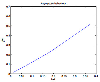
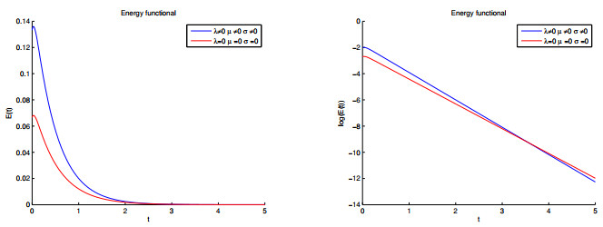
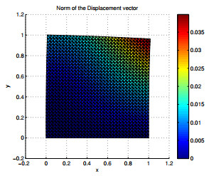
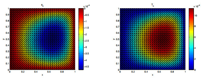
In this work, we study, from the numerical point of view, a dynamic thermoviscoelastic problem involving micropolar materials. The model leads to a linear system composed of parabolic partial differential equations for the displacements, the microrotation and the temperature. Its weak form is written as a linear system made of first-order variational equations, in terms of the velocity field, the microrotation speed and the temperature. Fully discrete approximations are introduced by using the finite element method and the implicit Euler scheme. A discrete stability property and a priori error estimates are proved, from which the linear convergence is derived under some additional regularity conditions. Finally, some two-dimensional numerical simulations are presented to demonstrate the accuracy of the approximation and the behavior of the solution.
- Micropolar materials,
- themoviscoelasticity,
- finite elements,
- a priori error analysis,
- numerical simulations
Citation: Noelia Bazarra, José R. Fernández, Ramón Quintanilla. Numerical analysis of a problem in micropolar thermoviscoelasticity[J]. Electronic Research Archive, 2022, 30(2): 683-700. doi: 10.3934/era.2022036

Related Papers:

Abstract

In this work, we study, from the numerical point of view, a dynamic thermoviscoelastic problem involving micropolar materials. The model leads to a linear system composed of parabolic partial differential equations for the displacements, the microrotation and the temperature. Its weak form is written as a linear system made of first-order variational equations, in terms of the velocity field, the microrotation speed and the temperature. Fully discrete approximations are introduced by using the finite element method and the implicit Euler scheme. A discrete stability property and a priori error estimates are proved, from which the linear convergence is derived under some additional regularity conditions. Finally, some two-dimensional numerical simulations are presented to demonstrate the accuracy of the approximation and the behavior of the solution.

References

[1]	W. Voigt, Theoretische Studien über die Elasticitätsverhältnisse der Krystalle, Abhandlungen der Königlichen Gesellschaft der Wissenschaften in Göttingen, 1887.
[2]	E. Cosserat, F. Cosserat, Théorie des corps déformables, Hermann, Paris, 1909. https://doi.org/10.1038/081067a0
[3]	A. C. Eringen, E. S. Suhubi, Non-linear theory of simple microelastic solids, part I, Int. J. Eng. Sci., 2 (1964), 189–203. https://doi.org/10.1016/0020-7225(64)90004-7 doi: 10.1016/0020-7225(64)90004-7
[4]	A. C. Eringen, E. S. Suhubi, Non-linear theory of simple microelastic solids, part II, Int. J. Eng. Sci., 2 (1964), 389–404. https://doi.org/10.1016/0020-7225(64)90017-5 doi: 10.1016/0020-7225(64)90017-5
[5]	A. C. Eringen, Linear theory of micropolar elasticity, J. Math. Mech., 15 (1966), 909–923. http://www.jstor.org/stable/24901442
[6]	W. Nowacki, Couple stresses in the theory of thermoelasticity I, Bull. Acad. Polon. Sci. Ser. Sci. Tech., 14 (1966), 129–138. https://doi.org/10.1007/978-3-7091-5581 doi: 10.1007/978-3-7091-5581
[7]	T. R. Tauchert, W. D. Claus, T. Ariman, The linear theory of micropolar thermoelasticity, Int. J. Eng. Sci., 76 (1968), 36–47. https://doi.org/10.1016/0020-7225(68)90037-2 doi: 10.1016/0020-7225(68)90037-2
[8]	T. R. Tauchert, Thermal stresses in micropolar elastic solids, Acta Mech., 11 (1971), 155–169. https://doi.org/10.1007/BF01176553 doi: 10.1007/BF01176553
[9]	R. S. Dhaliwal, A. Singh, Micropolar thermoelasticity, in Thermal Stresses II, Mechanical and mathematical methods (ed. R. Hetnarski), North-Holland, 1987.
[10]	A. C. Eringen, Microcontinuum Field Theories. I: Foundations and Solids, Springer-Verlag, New York, 1999. https://doi.org/10.1007/978-1-4612-0555-5
[11]	D. Ieşan, Thermoelastic models of continua, Solid Mechanics and Its Applications, 2004. https://doi.org/10.1007/978-1-4020-2310-1
[12]	A. S. El-Karamany, Uniqueness and reciprocity theorems in generalized linear micropolar thermoviscoelasticity, Int. J. Eng. Sci., 40 (2002), 2097–2117. https://doi.org/10.1016/S0020-7225(02)00142-8 doi: 10.1016/S0020-7225(02)00142-8
[13]	M. Aouadi, Temperature dependence of an elastic modulus in generalized linear micropolar thermoelasticity, Z. Angew. Math. Phys., 57 (2006), 1057–1074. https://doi.org/10.1007/s00033-005-0055-0 doi: 10.1007/s00033-005-0055-0
[14]	S. S. Aslanyan, S. H. Sargsyan, Applied theories of thermoelasticity of micropolar thin beams, J. Thermal Stresses, 41 (2018), 687–705. https://doi.org/10.1080/01495739.2018.1426066 doi: 10.1080/01495739.2018.1426066
[15]	D. S. Chandrasekharaiah, Variational and reciprocal principles in micropolar thermoelasticity, Int. J. Eng. Sci., 25 (1987), 55–63. https://doi.org/10.1016/0020-7225(87)90134-0 doi: 10.1016/0020-7225(87)90134-0
[16]	M. Ciarletta, A. Scalia, M. Svanadze, Fundamental solution in the theory of micropolar thermoelasticity for materials with voids, J. Thermal Stresses, 30 (2007), 213–229. https://doi.org/10.1080/01495730601130901 doi: 10.1080/01495730601130901
[17]	M. Ciarletta, M. Svanadze, L. Buonanno, Plane waves and vibrations in the theory of micropolar thermoelasticity for materials with voids, Eur. J. Mech. A/Solids, 28 (2009), 897–903. https://doi.org/10.1016/j.euromechsol.2009.03.008 doi: 10.1016/j.euromechsol.2009.03.008
[18]	A. S. El-Karamany, M. A. Ezzat, On the three-phase-lag linear micropolar thermoelasticity theory, Eur. J. Mech. A/Solids, 40 (2013), 198–208. https://doi.org/10.1016/j.euromechsol.2013.01.011 doi: 10.1016/j.euromechsol.2013.01.011
[19]	D. Ieşan, R. Quintanilla, On the grade consistent theory of micropolar thermoelasticity, J. Therm. Stresses, 15 (1992), 393–417. https://doi.org/10.1080/01495739208946146 doi: 10.1080/01495739208946146
[20]	S. Liu, Z. Si, Global well-posedness of the 3D micropolar equations with partial viscosity and damping, Appl. Math. Lett., 109 (2020), 106543. https://doi.org/10.1016/j.aml.2020.106543 doi: 10.1016/j.aml.2020.106543
[21]	F. Passarella, V. Zampoli, On the theory of micropolar thermoelasticity without energy dissipation, J. Therm. Stresses, 33 (2010), 305–317. https://doi.org/10.1080/014957399280760 doi: 10.1080/014957399280760
[22]	A. Pompei, M. A. Rigano, On the bending of micropolar viscoelastic plates, Int. J. Eng. Sci., 44 (2006), 1324–1333. https://doi.org/10.1016/j.ijengsci.2006.05.016 doi: 10.1016/j.ijengsci.2006.05.016
[23]	A. Scalia, A grade consistent micropolar theory of thermoelastic materials with voids, Z. Angew. Math. Mech. (ZAMM), 72 (1992), 133–140. https://doi.org/10.1002/zamm.19920720209 doi: 10.1002/zamm.19920720209
[24]	M. Svanadze, V. Tibullo, V. Zampoli, Fundamental solution in the theory of micropolar thermoelasticity without energy dissipation, J. Therm. Stresses, 29 (2006), 57–66. https://doi.org/10.1080/01495730500257417 doi: 10.1080/01495730500257417
[25]	W. E. Warren, E. Byskov, A general solution to some plane problems of micropolar elasticity, Eur. J. Mech. A/Solids, 27 (2008), 18–27. https://doi.org/10.1016/j.euromechsol.2007.05.006 doi: 10.1016/j.euromechsol.2007.05.006
[26]	A. Magaña, R. Quintanilla, On the uniqueness and analyticity of solutions in micropolar thermoviscoelasticity, J. Math. Anal. Appl., 412 (2014), 109–120. https://doi.org/10.1016/j.jmaa.2013.10.026 doi: 10.1016/j.jmaa.2013.10.026
[27]	M. A. Ezzat, A. S. El-Karamany, Fractional thermoelectric viscoelastic materials, J. Appl. Polyn. Sci., 124 (2012), 2187–2199. https://doi.org/10.1002/app.35243 doi: 10.1002/app.35243
[28]	M. A. Ezzat, A. S. El-Karamany, A. A. El-Bary, M. A. Fayik, Fractional calculus in one-dimensional isotropic thermo-viscoelasticity, Comptes Rendu Méc., 341 (2013), 553–566. https://doi.org/10.1016/j.crme.2013.04.001 doi: 10.1016/j.crme.2013.04.001
[29]	M. H. Hendy, M. M. Amin, M. A. Ezzat, Two-dimensional problem for thermoviscoelastic materials with fractional order heat transfer, J. Therm. Stresses, 42 (2019), 1298–1315. https://doi.org/10.1080/01495739.2019.1623734 doi: 10.1080/01495739.2019.1623734
[30]	P. G. Ciarlet, Basic error estimates for elliptic problems, in Handbook of Numerical Analysis (eds. P.G. Ciarlet and J.L. Lions), (1993), 17–351. https://doi.org/10.1016/S1570-8659(05)80039-0
[31]	M. Campo, J. R. Fernández, K. L. Kuttler, M. Shillor, J. M. Viaño, Numerical analysis and simulations of a dynamic frictionless contact problem with damage, Comput. Methods Appl. Mech. Eng., 196 (2006), 476–488. https://doi.org/10.1016/j.cma.2006.05.006 doi: 10.1016/j.cma.2006.05.006

Reader Comments

Your name:*

Email:*
© 2022 the Author(s), licensee AIMS Press. This is an open access article distributed under the terms of the Creative Commons Attribution License (http://creativecommons.org/licenses/by/4.0)