
Citation: Ebrahim Falahi, Zohre Delshadian, Hassan Ahmadvand, Samira Shokri Jokar. Head space volatile constituents and antioxidant properties of five traditional Iranian wild edible plants grown in west of Iran[J]. AIMS Agriculture and Food, 2019, 4(4): 1034-1053. doi: 10.3934/agrfood.2019.4.1034
[1] | Aini Ismafairus Abd Hamid, Nurfaten Hamzah, Siti Mariam Roslan, Nur Alia Amalin Suhardi, Muhammad Riddha Abdul Rahman, Faiz Mustafar, Hazim Omar, Asma Hayati Ahmad, Elza Azri Othman, Ahmad Nazlim Yusoff . Distinct neural mechanisms of alpha binaural beats and white noise for cognitive enhancement in young adults. AIMS Neuroscience, 2025, 12(2): 147-179. doi: 10.3934/Neuroscience.2025010 |
[2] | Tien-Wen Lee, Gerald Tramontano . Automatic parcellation of resting-state cortical dynamics by iterative community detection and similarity measurements. AIMS Neuroscience, 2021, 8(4): 526-542. doi: 10.3934/Neuroscience.2021028 |
[3] | David I. Dubrovsky . “The Hard Problem of Consciousness”. Theoretical solution of its main questions. AIMS Neuroscience, 2019, 6(2): 85-103. doi: 10.3934/Neuroscience.2019.2.85 |
[4] | Byron Bernal, Alfredo Ardila, Monica Rosselli . The Network of Brodmanns Area 22 in Lexico-semantic Processing: A Pooling-data Connectivity Study. AIMS Neuroscience, 2016, 3(3): 306-316. doi: 10.3934/Neuroscience.2016.3.306 |
[5] | Ioannis K Gallos, Kostakis Gkiatis, George K Matsopoulos, Constantinos Siettos . ISOMAP and machine learning algorithms for the construction of embedded functional connectivity networks of anatomically separated brain regions from resting state fMRI data of patients with Schizophrenia. AIMS Neuroscience, 2021, 8(2): 295-321. doi: 10.3934/Neuroscience.2021016 |
[6] | Zoha Deldar, Carlos Gevers-Montoro, Ali Khatibi, Ladan Ghazi-Saidi . The interaction between language and working memory: a systematic review of fMRI studies in the past two decades. AIMS Neuroscience, 2021, 8(1): 1-32. doi: 10.3934/Neuroscience.2021001 |
[7] | Matthew S. Sherwood, Jason G. Parker, Emily E. Diller, Subhashini Ganapathy, Kevin Bennett, Jeremy T. Nelson . Volitional down-regulation of the primary auditory cortex via directed attention mediated by real-time fMRI neurofeedback. AIMS Neuroscience, 2018, 5(3): 179-199. doi: 10.3934/Neuroscience.2018.3.179 |
[8] | Iliyan Ivanov, Kristin Whiteside . Dyadic Brain - A Biological Model for Deliberative Inference. AIMS Neuroscience, 2017, 4(4): 169-188. doi: 10.3934/Neuroscience.2017.4.169 |
[9] | Charles R Larson, Donald A Robin . Sensory Processing: Advances in Understanding Structure and Function of Pitch-Shifted Auditory Feedback in Voice Control. AIMS Neuroscience, 2016, 3(1): 22-39. doi: 10.3934/Neuroscience.2016.1.22 |
[10] |
M. Rosario Rueda, Joan P. Pozuelos, Lina M. Cómbita, Lina M. Cómbita .
Cognitive Neuroscience of Attention From brain mechanisms to individual differences in efficiency. AIMS Neuroscience, 2015, 2(4): 183-202. doi: 10.3934/Neuroscience.2015.4.183 |
Unfolding the complexity of the human brain function, as this is related to brain networking during cognitive tasks and/or at resting state, is one of the most significant and challenging research pursuits of our time. Depending on the questions asked, different connectivity modes may be sought [1]. For example, functional connectivity analysis seeks for statistical dynamic inter-dependencies between time series, while effective connectivity analysis seeks for causal-mechanistic influences that neural units exert to each other. On the other hand, structural connectivity seeks for anatomical connections between neuronal regions. Nevertheless, in the literature, a debate still exists considering the differences between effective and functional connectivity, and as a result, multiple definitions exist. In this work we follow the definition stated in Refs. [2], [3]. Towards the reconstruction of brain connectivity, various data-driven and model-driven approaches for mining the useful information included in datasets acquired by neuroimaging techniques such as Electroencephalography (EEG), Magnetoencephalography (MEG), Functional Magnetic Resonance Imaging (fMRI) and Positron Emission Tomography (PET) have been proposed (for a review see also [4], [5]). These extend from simple non-parametric methods such as correlation and coherence [6]–[9] to mutual information [10]–[13] and phase synchronization methods [14]–[17] and from linear data reduction methods such as Principal Component Analysis (PCA) and Independent Component Analysis (ICA) [18]–[20] to non-linear manifold learning methods such as ISOMAP [21], [22] and Diffusion Maps [23]. Parametric approaches include Granger-causality-based methods [24]–[29] and Dynamic Causal Modeling (DCM) for modelling the effective brain connectivity [30]. Relatively simple statistical approaches such as correlation and coherence analysis continue to hold a significant share in the modeling of brain (functional) connectivity of brain regions (see e.g. [8], [9]) especially on the basis of fMRI data [31], [32], however, these approaches fail in general to detect directional and multivariate dependencies. On the other hand, the concept of causality as introduced by Norbert Wiener [33] and formalized by Clive Granger [24] in economics has triggered significant further developments in neuroscience. According to the simplest form of Granger-causality (GC) a time-series X drives/influences another time series Y if past values of X help forecast better the evolution of Y as compared to using just the past values of Y. In its more general form, GC is performed on the basis of multivariate linear regression models. It has been applied in several studies, mainly in EEG and MEG [34]–[41]) but also in fMRI studies (see e.g. [42]–[53]).
GC is mainly a data-driven modeling approach for accessing functional connectivity that does not require any prior knowledge about the brain areas involved in a specific cognitive task. The (directed) interconnections between brain regions emerge from the statistical inter-dependencies between the corresponding emerged brain signals. On the the other hand, Dynamic Causal Modeling (DCM) is the most known representative method for reconstructing the underlying task-dependent effective connectivity from fMRI data and it is mainly model-driven [30], [54], [55]. In particular, it requires a prior knowledge (or guess) of the specific brain areas that are involved in the function of a specific cognitive task. DCM compares the efficiency of the various models (brain interconnections) under a Bayesian-based comparison to decide which model is the best in fitting the observed fMRI data. One of the advantages of DCM is that it inherently incorporates the experimental driving stimuli and modulatory inputs. For a a comparative evaluation and review of GC and DCM see Friston et al. [3].
Although GC could be in principle extended to find statistical dependencies from driving inputs (i.e. using multivariate autoregressive models with exogenous inputs (MVARX)) and furthermore identify modulatory effects on the functional connectivity network, only a very few number of studies have exploited this possibility (and even fewer in real experimental data). For example, Guo et al. [56] introduced partial GC and showed that partial GC cannot completely eliminate the influence of exogenous inputs and latent variables in all cases and that a complete elimination is only possible if “all common inputs have equal influence on all measured variables”. In their analysis, they considered various toy models with common exogenous inputs. They also considered the modelling of local field potential (LFP) data collected from the inferotemporal cortex of sheep; the (visual) stimulus signal was common to all electrodes. Roelstraete et al. [57] examined the efficiency of partial GC in the presence of none, weak and strong exogenous and latent variables. They concluded that in the presence of unknown latent and exogenous influences, the partial GC performs better than the conditional GC. The above studies examined the impact of exogenous inputs and latent influences on the efficiency of partial and conditional Granger, but they did not considered their identification/integration into the functional connectivity network. Alternatively, Ge et al. [58] proposed an extension of GC to handle exogenous inputs using a bilinear approximation similar to that of the DCM, in an attempt to incorporate the influence of external/experimental inputs. For the implementation of their approach, similarly to the DCM implementation, an a-priori knowledge of the specific regions that are driven by the input and/or the connections that are being modulated is assumed. In this respect, the development of extended GC schemes and the examination of their efficiency to deal with exogenous driving inputs and to identify the modulatory effects as those arise in real fMRI experiments is still an open problem. Towards this aim, Bajaj et al. [59] showed that non-parametric GC for pairwise calculations [60] and DCM give similar qualitative and quantitative results in the context of both simulated and real resting state fMRI.
In this work, we address an extended conditional MVGC modelling approach, which, apart from the emergent functional connectivity network reflecting the task-related brain organization, it identifies both the prominent stimulated regions driven by external stimuli and assess the impact of the modulation to the emerged interconnections. First, we present the extended GC modelling approach, and then we employ it to reconstruct the functional connectivity network based on stochastic synthetic data that involves external stimuli and modulation. Furthermore, we examine the impact of the haemodynamics in the inferred connectivity scheme. We then apply the proposed scheme to reconstruct the emergent functional connectivity network from a real fMRI experiment designed to investigate the role of the attention in the perception of the visual motion. This is a benchmark problem (see e.g. Ref. [59]) that has been exploited to validate various models within the DCM framework. We show that the proposed GC scheme results to a consistent connectivity pattern that compares well with the reference/best model obtained with the DCM approach and we also assess the computational cost of the methods.
The proposed methodology for the construction of the complete causality network that contains exogenous stimuli and modulatory inputs follows a three-tiered approach. In particular, in the first stage, we identify the emergent functional connectivity network using a multivariate (conditional) Granger causality (MVGC) analysis, without taking into account in the model, the presence of the exogenous and the modulatory inputs. At this point we should note that the emergent functional networks are different from the intrinsic cognitive networks i.e. the resting state networks (RSNs) [61], [62] that pertain to the activity of the brain in the absence of an external imposed task. When external stimuli are present, then the emergent (functional) connectivity network between brain regions is task-related and thus differs from the intrinsic resting-state activity. Hence, the time series reflecting the activity of the brain regions of the emergent task-related network will be more or less affected by the exogenous and modulatory inputs. However, it is expected that the exogenous/stimuli and modulatory input(s) will be more prominent, i.e. it will influence more the activity of particular region(s) and interconnections and that this will be reflected on larger values of causalities.
In the second stage, after the identification of the emergent functional connectivity network, we assess the influence that the exogenous input exerts on each one of the brain regions through a pairwise GC analysis. As discussed above, the hypothesis is that the exogenous inputs will affect more only one of the activated brain regions.
Finally in the third stage, the effect of modulatory inputs is assessed by formulating and solving an augmented MVGC problem. In the following sections we describe in detail the proposed approach.
In this section, we review the concepts of pairwise and conditional MVGC analysis for the construction of functional connectivity networks that are used for the construction of the emergent network as discussed above.
GC was initially introduced in 1969 by Clive Granger as a linear regression formalism of the idea of Wiener and Akaike
The magnitude of the GC that quantifies whether or not the full AR model is better than the restricted AR model in predicting the temporal evolution of the time series (i.e. that Yt(k) causes Yt(l)), (k, l = 1,2, k ≠ l) is defined as
where
Note that if
Thus, GC tests the null hypothesis:
In cases of indirect-joint influences between (groups of) more than two time series, the above “direct” pairwise-based formulation will provide spurious connections (see e.g. [60]). Take for example the paradigm of three groups of time series connected as shown in Figure 1, where the (group of) time series Yt(3) influences Yt(1) and consequently Yt(1) influences Yt(2). The pairwise GC may result to a statistically significant causality from Yt(3) to Yt(2).
Thus, when more than two regions are getting involved, it is required to access the conditional/multivariate GC (MVGC) [26], [28], [60], [63], [64].
Let us consider N (groups of) time series, and
For example for three (groups of) time series Y(l), Y(k), Y(m) the MVAR model reads:
The covariance matrix ∑M of the residual/ noise vectors et(l),et(k),et(m) is given by:
According to the above formulation, the conditional GC measure from Y(k) to Y(l) given/conditioned in (i.e. in the presence of) Y(m) is given by:
Here, we extend the above MVGC analysis, by considering an MVARX modeling approach in order to include exogenous inputs and assess the modulatory effects on the connectivity patterns. The first step of the approach is the reconstruction of the emergent connectivity (i.e. the functional connectivity resulting by excluding the exogenous inputs and modulations) based on the conventional MVGC analysis. In the second step, the scheme quantifies the influence of exogenous driving inputs (for example an experimentally designed visual or auditory stimulation) on each particular brain region involved in the given emergent connectivity network as computed in the first stage. Finally, the scheme access whether and where an exogenous modulatory signal influences the interconnections.
To begin with, we assume a deterministic known (experimentally designed) exogenous stimulus u(t) that acts on (excites) a particular brain region, out of n emergent inter-connected regions. The biophysical assumption here is that, the GC is directed from the exogenous driving signal to a particular brain region (which has to be identified). Let us inductively present the modelling approach by taking the time series Yt = {Y(1),Y(2),…Y(n)}∈Rn representing signals from n brain regions, while, at the same time, an exogenous input (a stimulus) u(t) is presented, though we do not know which brain region(s) this stimulus excites. We also assume that we have identified by MVGC the emergent functional connectivity network, i.e. we have constructed an MVAR model given by
For demonstration purposes, without the loss of generality, let us consider again three (groups of) time series Y(l), Y(k), Y(m). Then the corresponding MVARX model reads:
Thus, for the above MVARX, the GC that the exogenous input u(t) exerts in the (group of) region(s) Yi, i = l, k, m reads:
Thus, if
The above can be straightforwardly generalized to a network with n nodes and m driving inputs. In that case, for each exogeneous driving input we calculate n unidirectional conditional GCs (one for each node) and if, for instance, the i-th GC is not zero, we infer that the driving input acts on the i-th node (brain region). This analysis reveals which region is driven by a particular driving input.
Having constructed the emergent causal connectivity network (from the first stage of the approach) and assessed the effect of the exogenous input u (from the second stage of the approach), at the third stage we assess the impact of modulation on the emergent interconnections.
For our illustrations, let us consider one exogenous stimulus (u) and a modulatory input (v) acting on an emergent network involving three (brain) regions (see Figure 2) whose activity is represented by the time series Y(1), Y(2) and Y(2). In general, the modulatory input can influence any of the three emergent connections between the three regions. For the configuration shown in Figure (2), the modulatory input influences one of the three emergent connections marked with solid lines, there are three candidate MVARX models, which are given below.
Model A
Model B
Model C
Some of the regression coefficients in the above model depend on the modulatory input vt.
Now, each one of the equations that depend on the modulatory input (e.g.
Thus, by using the above transformation, the modulation of an external input v(t) is included in a new time series defined by
Finally,
Using the above formulation, we can now compute the corresponding measures for each one of the above models on the basis of the causalities that the new time series Y(i′) exert to the original time series Y(i).
For the above configuration the corresponding conditional GC (e.g. for Model A) reads:
where
If
In a system with n (groups of) brain regions, with one modulatory input v, one should estimate all possible combinations that match with the emergent connectivity scheme.
First, the performance of the proposed scheme is tested through a five-node network benchmark model (see e.g. Ref.
First, we performed a conditional MVGC analysis, using the Multivariate Granger Causality (MVGC) toolbox
Model orders | mean value | stand. deviation |
emergent connectivity | 2.96 | 0.20 |
Driving input | 2.84 | 0.37 |
Modulatory input (1′) | 2.67 | 0.47 |
Modulatory input (2′) | 2.92 | 0.27 |
Modulatory input (3′) | 2.89 | 0.31 |
Modulatory input (4′) | 2.74 | 0.44 |
Modulatory input (5′) | 2.63 | 0.49 |
As a next step, we estimated the GC from the driving input u(t) to each one of the internal time series Yt(i), i = 1,2,3,4,5. The results of this analysis are presented in
As a final step, we assessed the influence of the modulatory input vt. This step includes the generation of new five modified time series Yt(i′) = vtYt(i), i = 1,2,3,4,5, one for each of the five (see
In brief, the proposed scheme reconstructed successfully the actual connectivity pattern presented in Figure 3(a). The scheme succeeded also to reconstruct the actual networks for different/alternative configurations of the the driving and modulatory inputs.
In typical fMRI experiments the measured signals undergo haemodynamic latencies which are found to challenge the subsequent GC analysis [63]. For that reason, we also assessed the efficiency of the proposed analysis by considering haemodynamic latencies in the time series of the toy model of Figure 3(a). Actually, we convoluted the synthetic signals, produced by Eqs. (37), using canonical HRF functions, and then employed the proposed analysis onto the convoluted series; the convoluted time series were imported to MVGC toolbox for GC analysis. The considered HRFs are generated using the values of Ref. [66] which are based on experimentally observed data. As shown in Figure 4(a) the three considered canonical HRFs have different time-to-peak values, i.e., HRF-1 peaks at 3.8 s, while HRF-2 and HRF-3 peak at 5.7 and 7.7 s, respectively.
In these cases, the AIC used so far gives an almost 10-fold increased model order, while, on the other hand, the Bayesian Information Criterion (BIC) gives roughly a 4-fold increment. Consequently, in such, fMRI-like (HRF-convoluted) cases, it is more suitable to adopt the BIC for the estimation of the model order, as indicated also in Refs [27], [29], [63].
As a first step, we performed a GC analysis for the HRF-1 convoluted data set. The estimated model order (mean values and standard deviations) from 100 independent runs of each data set are shown in
Toy model with HRFs | mean value | stand. deviation |
Emergent connectivity - conv. HRF-1 | 12.59 | 0.68 |
Emergent connectivity - conv. HRF-2 | 17.17 | 1.01 |
Emergent connectivity - conv. HRF-3 | 22.02 | 1.38 |
– | – | – |
Driving input - conv. HRF-1 | 13.6 | 1.77 |
Driving input - conv. HRF-2 | 20.10 | 0.33 |
Driving input - conv. HRF-3 | 21.61 | 0.84 |
– | – | – |
Modulatory input (1′) - conv. HRF-1 | 12.11 | 0.55 |
Modulatory input (2′) - conv. HRF-1 | 11.97 | 0.50 |
Modulatory input (3′) - conv. HRF-1 | 12.06 | 0.57 |
Modulatory input (4′) - conv. HRF-1 | 12.03 | 0.48 |
Modulatory input (5′) - conv. HRF-1 | 12.04 | 0.37 |
Modulatory input (1′) - conv. HRF-2 | 16.48 | 0.86 |
Modulatory input (2′) - conv. HRF-2 | 16.46 | 0.64 |
Modulatory input (3′) - conv. HRF-2 | 16.36 | 0.60 |
Modulatory input (4′) - conv. HRF-2 | 16.40 | 0.65 |
Modulatory input (5′) - conv. HRF-2 | 16.46 | 0.70 |
Modulatory input (1′) - conv. HRF-3 | 21.06 | 1.50 |
Modulatory input (2′) - conv. HRF-3 | 20.76 | 1.80 |
Modulatory input (3′) - conv. HRF-3 | 20.85 | 1.40 |
Modulatory input (4′) - conv. HRF-3 | 20.82 | 1.55 |
Modulatory input (5′) - conv. HRF-3 | 20.77 | 1.22 |
As a next step, we applied the proposed scheme to access the impact of haemodynamic convolution with respect to the driving input. The estimated model orders for each case are shown in
The role of the attention in the perception of visual motion has been extensively studied using fMRI [67], [68]. In their landmark work, C. Buchel and K. Friston [67] using DCM showed that attention modulates the connectivity between brain regions involved in the perception of visual motion. In the present work, we analyzed the same fMRI dataset ([67]) which has served as benchmark problem in many studies [30], [54], [69]. The dataset was downloaded from the official SPM website (http://www.fil.ion.ucl.ac.uk/spm/data/attention/), where the fMRI data are smoothed, spatially normalized, realigned, and slice-time corrected. As described in Ref. [67], in the original experiment the subjects were observing a black computer screen displaying white dots. According to the experimental design, there where specific epochs, where the dots where either static or moving. Intermediate epochs without dots and only one static picture were also introduced. In several epochs of moving dots, the subjects were instructed to keen on possible changes in the velocity of the moving dots, although no changes really existed. Therefore, three experimental variables are considered: photic for visual stimulation, motion for moving dots, and attention for the observation of possible changes in the velocity of the dots. Following Refs. [67]–[69], we identified three activated brain regions, namely the V1, V5 and SPC, and extracted the corresponding time series through eigendecomposition [67], using the Statistical Parametric Mapping toolbox (SPM12) [70]–[72]. In previous works, the aforementioned connectivity network had been intensively investigated using the DCM method [54], [69].
Here, we applied, the proposed extended GC analysis, to infer the underlying connectivity network. The extracted time series for each brain region involved in this task are shown in Figure 6(a). By importing the three extracted time series (V1, V5 and SPC) into the MVGC toolbox, we obtained the emerging connectivity matrix shown in Figure 6(b).
The model order, according to BIC is 1, which can be attributed to the low sampling rate of the particular fMRI data
As a next step, we sought to associate the external visual stimuli (driving input) with one of the brain regions involved. In this respect, we estimated the causal effect of the Photic time series, shown in
Finally, to complete the circuit diagram, we assessed the modulatory effect of two inputs, namely that of motion and attention, whose time series are shown in
Finally, in order to assess the validity of the resulted network, we compared the inferred model (shown again in Figure 8(a) (model 1)) with an alternative model (model 2) taken from Refs. [54], [69]. In particular, model 2, shown in Figure 8(b) is the reference selected model, obtained in Refs. [54], [69] as the best among other candidate models using DCM analysis. The two models differ with respect to the emergent connections between regions V1 and SPC, and between V5 and SPC. Furthermore, model 1 assumes that the modulatory inputs affect more connections. Here, we compared their posterior likelihood through bayesian model selection by importing the two models into the SPM12 software [70]–[72]. The log-evidence (see Ref. [54] for details) for model 1 is found −3221, while for model 2 equals to −3285. Therefore, the natural logarithm of the Bayes factor B12 equals to 64 suggesting that the data favour model 1 over model 2. We note here, that the net computational time for deducing model 1 using the proposed GC analysis, is less than five seconds, using an i7 processor and 32 GiB RAM. On the other hand, model 2 was taken from Refs. [54], [69] ready-made. However, as detailed in Refs. [54], [69], deducing model 2 requires a prior knowledge, and then, a Bayesian comparison is applied between pairs of alternative models. Since each Bayesian comparison requires one-minute computational time using the aforementioned machine, it comes out that the respective cost is dramatically increased compared to that of GC inference, especially when all possible configurations are included, as shown also in Ref. [73] for typical GC and dynamic-Byesian inference in larger networks.
Granger causality (GC) and Dynamic causal modelling (DCM) are the two key methodologies for the reconstruction of directed connectivity patterns of brain functioning. GC is considered as a generic data-driven approach that is mostly used for the reconstruction of the emergent functional connectivity (brain regions interconnected in terms of statistical dependence) without dealing with the modelling and influence of exogenous and/or modulatory inputs on the network structure. On the other hand, DCM has been mostly used to infer the effective connectivity from task-related fMRI data enabling the selection of specific models (network structures). For a critical discussion on the analysis of connectivity with GC and DCM one can refer to Friston et al. [3]. One of the main points raised in this paper is that GC and DCM are complementary and that GC can in principle be used to provide candidate models for DCM, thus enhancing our ability to better model and understand cognitive integration. However, to date, only very few studies have investigated this possibility. For example, Bajaj et al. [59] compared the performance of GC and DCM using both synthetic and real resting-state fMRI data. They found that both methods result to consistent directed functional and effective connectivity patterns. Here, we proposed an extension of the conditional MVGC to deal with task-related fMRI data with exogenous/driving and modulatory inputs. Based on both synthetic and real task-related fMRI data, we showed that the proposed GC scheme successfully identifies the functional connectivity patterns. We also show that the computational time that is needed with the proposed scheme is much less compared to DCM. The key-stones of two methods, i.e. their origin and the results that are obtained based on their use are different. Here, we summarize the pros and cons of the two approaches. GC stems out the theory of time-series analysis, and specifically of the model identification of MVAR models, and it is used to provide directed functional connectivity, that is statistical dependence between neuronal systems based on various neuroimaging techniques (mainly EEG, but also MEG and fMRI). On the other hand, DCM is based on a bio-physical modelling approach, targeting at revealing the effective direct connectivity between brain regions from fMRI data. GC has been mostly used until now to detect the emergent functional connectivity networks, i.e. the functional conenctivity networks that emerge due to inputs but without modelling them. Our approach aims to resolve this issue. On the other hand, DCM handles explicitly such information. GC offers a general black-box framework, which is relatively computational cheap when dealing with small to medium dimension of data, while DCM is a framework that is based more on a-priori knowledge about the neuronal system under study and finds the best models from a set of plausible model using hypothesis testing and is more computational demanding as it is based on realistic biophysical modelling. Thus, differences in the connectivity networks found by the two methods should be attributed to the above different origins and capabilities. For a detailed review of the pros and cons of GC and DCM one can refer to the paper of Friston [3]. All in all, GC and DCM should not be considered as two opponent approaches, but rather as complementary. Thus, our results suggest that the proposed GC scheme may be used as stand-alone and/or complementary approach to DCM to provide new candidate models for DCM for furthe analysis and comparisons.
[1] | Sharafzadeh S, Alizadeh O (2012) Some medicinal plants cultivated in Iran. J Appl Pharm Sci 2: 134-7. |
[2] | Nikbakht A, Kafi M, Haghighi M (2004) The abilities and potentials of medicinal plants production and herbal medicine in Iran. VIIIth International People-Plant Symposium on Exploring Therapeutic Powers of Flowers, Greenery and Nature, 790: 259-262. |
[3] | Mathew NT (2001) Pathophysiology, epidemiology, and impact of migraine. Clin cornerstone 4: 1-17. |
[4] |
Lobo V, Patil A, Phatak A, et al. (2010) Free radicals, antioxidants and functional foods: Impact on human health. Pharmacogn Rev 4: 118. doi: 10.4103/0973-7847.70902
![]() |
[5] |
Huang WY, Cai YZ, Zhang Y (2009) Natural phenolic compounds from medicinal herbs and dietary plants: potential use for cancer prevention. Nutr Cancer 62: 1-20. doi: 10.1080/01635580903191585
![]() |
[6] |
Scheibmeir HD, Christensen K, Whitaker SH, et al. (2005) A review of free radicals and antioxidants for critical care nurses. Intensive Criti Care Nurs 21: 24-8. doi: 10.1016/j.iccn.2004.07.007
![]() |
[7] |
Tachakittirungrod S, Okonogi S, Chowwanapoonpohn S (2007) Study on antioxidant activity of certain plants in Thailand: Mechanism of antioxidant action of guava leaf extract. Food Chem 103: 381-8. doi: 10.1016/j.foodchem.2006.07.034
![]() |
[8] | Ahmadvand H, Amiri H, Dalvand H, et al. (2014) Various antioxidant properties of essential oil and hydroalcoholic extract of Artemisa persica. J Birjand Univ Med Sci 20: 416-424 [In Persian]. |
[9] |
El-Ghorab A, El-Massry KF, Shibamoto T (2007) Chemical composition of the volatile extract and antioxidant activities of the volatile and nonvolatile extracts of Egyptian corn silk (Zea mays L.). J Agric Food Chem 55: 9124-7. doi: 10.1021/jf071646e
![]() |
[10] |
Mimaki Y, Kuroda M, Fukasawa T, et al. (1999) Steroidal glycosides from the bulbs of Allium jesdianum. J Nat prod 62: 194-197. doi: 10.1021/np980346b
![]() |
[11] | Grases F, Prieto RM, Gomila I, et al. (2009) Phytotherapy and renal stones: the role of antioxidants. A pilot study in Wistar rats. Urol Res 37: 35. |
[12] |
Nair MP, Mahajan S, Reynolds JL, et al. (2006) The flavonoid quercetin inhibits proinflammatory cytokine (tumor necrosis factor alpha) gene expression in normal peripheral blood mononuclear cells via modulation of the NF-κβ system. Clin Vaccine Immunol 13: 319-28. doi: 10.1128/CVI.13.3.319-328.2006
![]() |
[13] | Hossini S, Mohammadi J, Delaviz H, et al. (2017) Protective effect of hydroalcoholic extract of Nasturtium Officinalis against carbon tetrachloride-induced liver damage in rats. Armaghan-e-Danesh 22: 674-85 [In Persian]. |
[14] |
Goda Y, Hoshino K, Akiyama H, et al. (1999) Constituents in watercress: inhibitors of histamine release from RBL-2H3 cells induced by antigen stimulation. Biol Pharm Bull 22: 1319-26. doi: 10.1248/bpb.22.1319
![]() |
[15] | Chung F, Morse M, Eklind K, et al. (1992) Quantitation of human uptake of the anticarcinogen phenethyl isothiocyanate after a watercress meal. Cancer Epidemiol Prev Biomark 1: 383-8. |
[16] | Getahun SM, Chung FL (1999) Conversion of glucosinolates to isothiocyanates in humans after ingestion of cooked watercress. Cancer Epidemiol Prev Biomark 8: 447-51. |
[17] | Ahvazi M, Khalighi-Sigaroodi F, Charkhchiyan MM, et al. (2012) Introduction of medicinal plants species with the most traditional usage in Alamut region. Iran J Pharm Res: IJPR 11: 185. |
[18] | Mohammadi J, Motlagh FT, Mohammadi N (2017) The effect of hydroalcoholic extract of watercress on parameters of reproductive and sex hormones on the diabetic rats. J Pharm Sci Res 9: 1334. |
[19] |
Martínez-Sánchez A, Gil-Izquierdo A, Gil MI, et al. (2008) comparative study of flavonoid compounds, vitamin C, and antioxidant properties of baby leaf Brassicaceae species. J Agric Food Chem 56: 2330-40. doi: 10.1021/jf072975+
![]() |
[20] |
Bahramikia S, Ardestani A, Yazdanparast R (2009) Protective effects of four Iranian medicinal plants against free radical-mediated protein oxidation. Food Chem 115: 37-42. doi: 10.1016/j.foodchem.2008.11.054
![]() |
[21] | Ozen T (2009) Investigation of antioxidant properties of Nasturtium officinale (watercress) leaf extracts. Acta Pol Pharm 66: 187-93. |
[22] |
Amiri H (2012) Volatile constituents and antioxidant activity of flowers, stems and leaves of Nasturtium officinale R. Br. Nat Prod Res 26: 109-15. doi: 10.1080/14786419.2010.534998
![]() |
[23] |
Park NI, Kim JK, Park WT, et al. (2011) An efficient protocol for genetic transformation of watercress (Nasturtium officinale) using Agrobacterium rhizogenes. Mol Biol Rep 38: 4947-53. doi: 10.1007/s11033-010-0638-5
![]() |
[24] | Akila M, Devaraj H (2008) Synergistic effect of tincture of Crataegus and Mangifera indica L. extract on hyperlipidemic and antioxidant status in atherogenic rats. Vasc Pharmacol 49: 173-7. |
[25] | Tosun M, Ercisli S, Ozer H, et al. (2012) Chemical composition and antioxidant activity of foxtail lily (Eremurus spectabilis). Acta Sci Pol Hortorum Cultus 11: 145-53. |
[26] | Baytop T (1984) Türkiye'de Bitkiler ile Tedavi, İstanbul Üniv. Eczacılık Fak Yayınları. |
[27] | Farzaei MH, Rahimi R, Attar F, et al. (2014) Chemical composition, antioxidant and antimicrobial activity of essential oil and extracts of Tragopogon graminifolius, a medicinal herb from Iran. Nat Prod Commun 9: 1934578X1400900134. |
[28] |
Guarrera PM (2003) Food medicine and minor nourishment in the folk traditions of Central Italy (Marche, Abruzzo and Latium). Fitoter 74: 515-44. doi: 10.1016/S0367-326X(03)00122-9
![]() |
[29] |
Singh K, Lal B (2008) Ethnomedicines used against four common ailments by the tribal communities of Lahaul-Spiti in western Himalaya. J Ethnopharmacol 115: 147-59. doi: 10.1016/j.jep.2007.09.017
![]() |
[30] | Farzaei MH, Khazaei M, Abbasabadei Z, et al. (2013) Protective effect of tragopogon graminifolius DC against ethanol induced gastric ulcer. Iran Red Crescent Med J 15: 813. |
[31] |
Farzaei MH, Rahimi R, Abbasabadi Z, et al. (2013) An evidence-based review on medicinal plants used for the treatment of peptic ulcer in traditional Iranian medicine. Int J Pharmacol 9: 108-124. doi: 10.3923/ijp.2013.108.124
![]() |
[32] | Hamideh J, Khosro P, Javad NDM (2012) Callus induction and plant regeneration from leaf explants of Falcaria vulgaris an important medicinal plant. J Med Plants Res 6: 3407-14. |
[33] | Shafaghat A (2010) Free radical scavenging and antibacterial activities, and GC/MS analysis of essential oils from different parts of Falcaria vulgaris from two regions. Nat Prod Commun 5: 1934578X1000500636. |
[34] |
Erkan N, Akgonen S, Ovat S, et al. (2011) Phenolic compounds profile and antioxidant activity of Dorystoechas hastata L. Boiss et Heldr. Food Res Int 44: 3013-20. doi: 10.1016/j.foodres.2011.07.015
![]() |
[35] |
Mulinacci N, Innocenti M, Bellumori M, et al. (2011) Storage method, drying processes and extraction procedures strongly affect the phenolic fraction of rosemary leaves: an HPLC/DAD/MS study. Talanta 85: 167-76. doi: 10.1016/j.talanta.2011.03.050
![]() |
[36] |
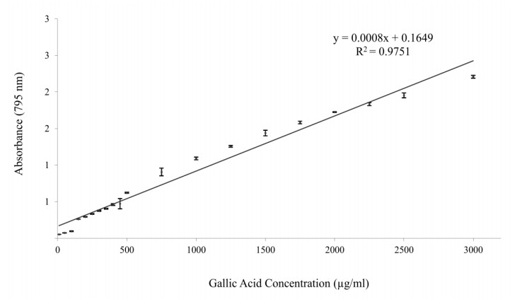
Singleton VL, Orthofer R, Lamuela-Raventós RM, et al. (1999) Analysis of total phenols and other oxidation substrates and antioxidants by means of folin-ciocalteu reagent. Methods Enzymol 299: 152-78. doi: 10.1016/S0076-6879(99)99017-1
![]() |
[37] |
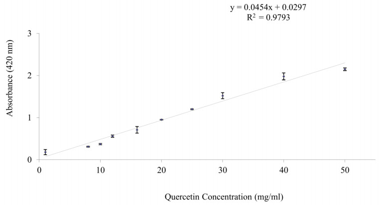
Woisky RG, Salatino A (1998) Analysis of propolis: some parameters and procedures for chemical quality control. J Apic Res 37: 99-105. doi: 10.1080/00218839.1998.11100961
![]() |
[38] | Ahmadvand H, Amiri H, Dalvand H (2015) Antioxidant properties of hydro-alcoholic extract and extract of nepeta crispa in Lorestan province. Hormozgan Med J 19: 172-9. |
[39] |
Duthie G, Crozier A (2000) Plant-derived phenolic antioxidants. Curr Opin Lipidol 11: 43-7. doi: 10.1097/00041433-200002000-00007
![]() |
[40] |
Karaman K, Polat B, Ozturk I, et al. (2011) Volatile compounds and bioactivity of Eremurus spectabilis (Ciris), a Turkish wild edible vegetable. J Med Food 14: 1238-43. doi: 10.1089/jmf.2010.0262
![]() |
[41] | Murathan ZT, Arslan M, Erbil N (2018) Evaluation of antioxidant, antimicrobial and antimutagenic properties in eremurus spectabilis bieb. grown in different ecological regions. Fresenius Environ Bull 27: 9491-9. |
[42] | Pourfarzad A, Hadad KMH, Habibi NMB, et al. (2013) Efficacy of ultrasound in the extraction of fructan from tubers of Eremurus spectabilis using Box-Behnken design. J Res Innov Food Technol 2: 219. |
[43] |
Boligon AA, Janovik V, Boligon AA, et al. (2013) HPLC analysis of polyphenolic compounds and antioxidant activity in Nasturtium officinale. Int J Food Prop 16: 61-9. doi: 10.1080/10942912.2010.528111
![]() |
[44] |
Yazdanparast R, Bahramikia S, Ardestani A (2008) Nasturtium officinale reduces oxidative stress and enhances antioxidant capacity in hypercholesterolaemic rats. Chem Biol Interact 172: 176-84. doi: 10.1016/j.cbi.2008.01.006
![]() |
[45] |
Gill CI, Haldar S, Boyd LA, et al. (2007) Watercress supplementation in diet reduces lymphocyte DNA damage and alters blood antioxidant status in healthy adults. Am J Clin Nutr 85: 504-10. doi: 10.1093/ajcn/85.2.504
![]() |
[46] | Potter JD, Steinmetz K (1996) Vegetables, fruit and phytoestrogens as preventive agents. IARC Sci Publ 61-90. |
[47] |
Verhoeven DT, Verhagen H, Goldbohm RA, et al. (1997) Review of mechanisms underlying anticarcinogenicity by brassica vegetables. Chem Biol Interac 103: 79-129. doi: 10.1016/S0009-2797(96)03745-3
![]() |
[48] |
Lhoste E, Gloux K, De Waziers I, et al. (2004) The activities of several detoxication enzymes are differentially induced by juices of garden cress, water cress and mustard in human HepG2 cells. Chem Biol Interac 150: 211-9. doi: 10.1016/j.cbi.2004.08.007
![]() |
[49] | Mazandarani M, Momeji A, Zarghami MP (2013) Evaluation of phytochemical and antioxidant activities from different parts of Nasturtium officinale R. Br. in Mazandaran. Iran J Plant Physiol 3: 659-664. |
[50] |
Ghasemi Pirbalouti A, Siahpoosh A, Setayesh M, et al. (2014) Antioxidant activity, total phenolic and flavonoid contents of some medicinal and aromatic plants used as herbal teas and condiments in Iran. J Med Food 17: 1151-7. doi: 10.1089/jmf.2013.0057
![]() |
[51] | Pourmorad F, Hosseinimehr S, Shahabimajd N (2006) Antioxidant activity, phenol and flavonoid contents of some selected Iranian medicinal plants. Afr J Biotechnol 5: 1142-1145. |
[52] |
Nickavar B, Esbati N (2012) Evaluation of the antioxidant capacity and phenolic content of three Thymus species. J Acupunct Meridian Stud 5: 119-25. doi: 10.1016/j.jams.2012.03.003
![]() |
[53] |
Ghasemzadeh A, Jaafar HZ, Rahmat A (2010) Antioxidant activities, total phenolics and flavonoids content in two varieties of Malaysia young ginger (Zingiber officinale Roscoe). Mol 15: 4324-33. doi: 10.3390/molecules15064324
![]() |
[54] |
Maisuthisakul P, Suttajit M, Pongsawatmanit R (2007) Assessment of phenolic content and free radical-scavenging capacity of some Thai indigenous plants. Food Chem 100: 1409-18. doi: 10.1016/j.foodchem.2005.11.032
![]() |
[55] |
Kähkönen MP, Hopia AI, Vuorela HJ, et al (1999) Antioxidant activity of plant extracts containing phenolic compounds. J Agric Food Chem 47: 3954-62. doi: 10.1021/jf990146l
![]() |
[56] |
Yu L, Haley S, Perret J, et al. (2002) Free radical scavenging properties of wheat extracts. J Agric Food Chem 50: 1619-24. doi: 10.1021/jf010964p
![]() |
[57] |
Surveswaran S, Cai YZ, Corke H, et al. (2007) Systematic evaluation of natural phenolic antioxidants from 133 Indian medicinal plants. Food Chem 102: 938-53. doi: 10.1016/j.foodchem.2006.06.033
![]() |
[58] |
Kaur C, Kapoor HC (2002) Anti‐oxidant activity and total phenolic content of some Asian vegetables. Int J Food Sci Technol 37: 153-61. doi: 10.1046/j.1365-2621.2002.00552.x
![]() |
[59] |
Wong SP, Leong LP, Koh JHW (2006) Antioxidant activities of aqueous extracts of selected plants. Food Chem 99: 775-83. doi: 10.1016/j.foodchem.2005.07.058
![]() |
[60] |
Huang B, Lei Y, Tang Y, et al. (2011) Comparison of HS-SPME with hydrodistillation and SFE for the analysis of the volatile compounds of Zisu and Baisu, two varietal species of Perilla frutescens of Chinese origin. Food Chem 125: 268-75. doi: 10.1016/j.foodchem.2010.08.043
![]() |
[61] | Akthar MS, Degaga B, Azam T (2014) Antimicrobial activity of essential oils extracted from medicinal plants against the pathogenic microorganisms: a review. Issues Biol Sci Pharm Res 2: 1-7. |
[62] |
Calo JR, Crandall PG, O'Bryan CA, et al. (2015) Essential oils as antimicrobials in food systems-A review. Food Control 54: 111-9. doi: 10.1016/j.foodcont.2014.12.040
![]() |
[63] |
Gonzalez-Burgos E, Gomez-Serranillos M (2012) Terpene compounds in nature: A review of their potential antioxidant activity. Curr Med Chem 19: 5319-41. doi: 10.2174/092986712803833335
![]() |
[64] |
Paduch R, Kandefer-Szerszeń M, Trytek M, et al. (2007) Terpenes: substances useful in human healthcare. Arch Immunol Ther Exp 55: 315. doi: 10.1007/s00005-007-0039-1
![]() |
[65] |
Dawidowicz AL, Olszowy M (2010) Influence of some experimental variables and matrix components in the determination of antioxidant properties by β-carotene bleaching assay: experiments with BHT used as standard antioxidant. Eur Food Res Technol 231: 835-40. doi: 10.1007/s00217-010-1333-4
![]() |
[66] |
Dekker M, Verkerk R, Van Der Sluis A, et al. (1999) Analysing the antioxidant activity of food products: processing and matrix effects. Toxicology in vitro 13: 797-9. doi: 10.1016/S0887-2333(99)00057-0
![]() |
[67] |
Parada J, Aguilera J (2007) Food microstructure affects the bioavailability of several nutrients. J Food Sci 72: R21-R32. doi: 10.1111/j.1750-3841.2007.00274.x
![]() |
[68] |
Xu DP, Li Y, Meng X, et al. (2017) Natural antioxidants in foods and medicinal plants: Extraction, assessment and resources. Int J Mol Sci 18: 96. doi: 10.3390/ijms18010096
![]() |
1. | Chaojun Zhang, Yunling Ma, Lishan Qiao, Limei Zhang, Mingxia Liu, Learning functional brain networks with heterogeneous connectivities for brain disease identification, 2024, 180, 08936080, 106660, 10.1016/j.neunet.2024.106660 | |
2. | Ioannis K. Gallos, Daniel Lehmberg, Felix Dietrich, Constantinos Siettos, Data-driven modelling of brain activity using neural networks, diffusion maps, and the Koopman operator, 2024, 34, 1054-1500, 10.1063/5.0157881 | |
3. | Lina Jia, Hua Jin, Xiaokang Jin, Neural mechanisms of the continued influence effect of misinformation: Analysis based on fMRI causal connectivity, 2024, 836, 03043940, 137861, 10.1016/j.neulet.2024.137861 |
Model orders | mean value | stand. deviation |
emergent connectivity | 2.96 | 0.20 |
Driving input | 2.84 | 0.37 |
Modulatory input (1′) | 2.67 | 0.47 |
Modulatory input (2′) | 2.92 | 0.27 |
Modulatory input (3′) | 2.89 | 0.31 |
Modulatory input (4′) | 2.74 | 0.44 |
Modulatory input (5′) | 2.63 | 0.49 |
Toy model with HRFs | mean value | stand. deviation |
Emergent connectivity - conv. HRF-1 | 12.59 | 0.68 |
Emergent connectivity - conv. HRF-2 | 17.17 | 1.01 |
Emergent connectivity - conv. HRF-3 | 22.02 | 1.38 |
– | – | – |
Driving input - conv. HRF-1 | 13.6 | 1.77 |
Driving input - conv. HRF-2 | 20.10 | 0.33 |
Driving input - conv. HRF-3 | 21.61 | 0.84 |
– | – | – |
Modulatory input (1′) - conv. HRF-1 | 12.11 | 0.55 |
Modulatory input (2′) - conv. HRF-1 | 11.97 | 0.50 |
Modulatory input (3′) - conv. HRF-1 | 12.06 | 0.57 |
Modulatory input (4′) - conv. HRF-1 | 12.03 | 0.48 |
Modulatory input (5′) - conv. HRF-1 | 12.04 | 0.37 |
Modulatory input (1′) - conv. HRF-2 | 16.48 | 0.86 |
Modulatory input (2′) - conv. HRF-2 | 16.46 | 0.64 |
Modulatory input (3′) - conv. HRF-2 | 16.36 | 0.60 |
Modulatory input (4′) - conv. HRF-2 | 16.40 | 0.65 |
Modulatory input (5′) - conv. HRF-2 | 16.46 | 0.70 |
Modulatory input (1′) - conv. HRF-3 | 21.06 | 1.50 |
Modulatory input (2′) - conv. HRF-3 | 20.76 | 1.80 |
Modulatory input (3′) - conv. HRF-3 | 20.85 | 1.40 |
Modulatory input (4′) - conv. HRF-3 | 20.82 | 1.55 |
Modulatory input (5′) - conv. HRF-3 | 20.77 | 1.22 |