In this paper, we consider a system of reaction-diffusion equations in a domain consisting of two bulk regions separated by a thin layer with thickness of order $ε$ and a periodic heterogeneous structure. The equations inside the layer depend on $ε$ and the diffusivity inside the layer on an additional parameter $γ ∈ [-1, 1]$. On the bulk-layer interface, we assume a nonlinear Neumann-transmission condition depending on the solutions on both sides of the interface. For $\epsilon \to0 $, when the thin layer reduces to an interface $Σ$ between two bulk domains, we rigorously derive macroscopic models with effective conditions across the interface $Σ$. The crucial part is to pass to the limit in the nonlinear terms, especially for the traces on the interface between the different compartments. For this purpose, we use the method of two-scale convergence for thin heterogeneous layers, and a Kolmogorov-type compactness result for Banach valued functions, applied to the unfolded sequence in the thin layer.
Citation: Markus Gahn, Maria Neuss-Radu, Peter Knabner. Effective interface conditions for processes through thin heterogeneous layers with nonlinear transmission at the microscopic bulk-layer interface[J]. Networks and Heterogeneous Media, 2018, 13(4): 609-640. doi: 10.3934/nhm.2018028
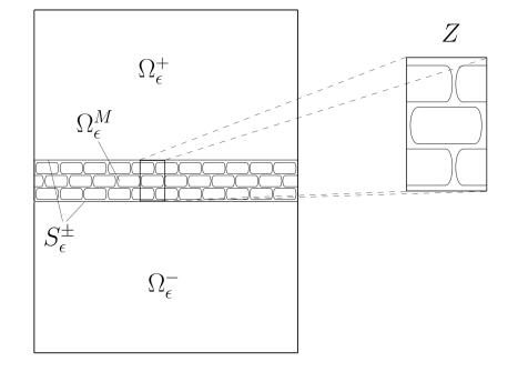
In this paper, we consider a system of reaction-diffusion equations in a domain consisting of two bulk regions separated by a thin layer with thickness of order $ε$ and a periodic heterogeneous structure. The equations inside the layer depend on $ε$ and the diffusivity inside the layer on an additional parameter $γ ∈ [-1, 1]$. On the bulk-layer interface, we assume a nonlinear Neumann-transmission condition depending on the solutions on both sides of the interface. For $\epsilon \to0 $, when the thin layer reduces to an interface $Σ$ between two bulk domains, we rigorously derive macroscopic models with effective conditions across the interface $Σ$. The crucial part is to pass to the limit in the nonlinear terms, especially for the traces on the interface between the different compartments. For this purpose, we use the method of two-scale convergence for thin heterogeneous layers, and a Kolmogorov-type compactness result for Banach valued functions, applied to the unfolded sequence in the thin layer.

| [1] |
Homogenization and two-scale convergence. SIAM J. Math. Anal. (1992) 23: 1482-1518. 
|
| [2] |
Derivation of the double porosity model of single phase flow via homogenization theory. SIAM J. Math. Anal. (1990) 27: 823-836.
|
| [3] |
Modelling of an underground waste disposal site by upscaling. Math. Meth. Appl. Sci. (2004) 27: 381-403.
|
| [4] |
A homogenized model of an underground waste repository including a disturbed zone. Multiscale Model. Simul. (2005) 3: 918-939.
|
| [5] | H. Brezis, Functional Analysis, Sobolev Spaces and Partial Differential Equations, Springer-Verlag, New York, 2011. |
| [6] |
The periodic unfolding method in homogenization. SIAM J. Math. Anal. (2008) 40: 1585-1620.
|
| [7] |
The periodic unfolding method for perforated domains and Neumann sieve models. J. Math. Pures Appl. (2008) 89: 248-277.
|
| [8] | A characterization of relatively compact sets in Lp(Ω, B). Stud. Univ. Babeş-Bolyai Math. (2016) 61: 279-290. |
| [9] |
Homogenization of reaction-diffusion processes in a two-component porous medium with nonlinear flux conditions at the interface. SIAM Journal on Applied Mathematics (2016) 76: 1819-1843.
|
| [10] |
Derivation of effective transmission conditions for domains separated by a membrane for different scaling of membrane diffusivity. Discrete & Continuous Dynamical Systems-Series S (2017) 10: 773-797.
|
| [11] |
Homogenization via unfolding in periodic layer with contact. Asymptotic Analysis (2016) 99: 23-52.
|
| [12] |
Asymptotic analysis for domains separated by a thin layer made of periodic vertical beams. Journal of Elasticity (2017) 128: 291-331.
|
| [13] | Homogenization of non-linear variational problems with thin inclusions. Math. J. Okayama Univ. (2012) 54: 97-131. |
| [14] | M. Neuss-Radu, Mathematical modelling and multi-scale analysis of transport processes through membranes (habilitation thesis), University of Heidelberg, 2017. |
| [15] |
Effective transmission conditions for reaction-diffusion processes in domains separated by an interface. SIAM J. Math. Anal. (2007) 39: 687-720.
|
| [16] |
A general convergence result for a functional related to the theory of homogenization. SIAM J. Math. Anal. (1989) 20: 608-623.
|
| [17] |
Analysis and upscaling of a reactive transport model in fractured porous media with nonlinear transmission condition. Vietnam Journal of Mathematics (2017) 45: 77-102.
|
| [18] | C. Vogt, A Homogenization Theorem Leading to a Volterra Integro-Differential Equation for Permeation Chromotography, SFB 123, University of Heidelberg, Preprint 155 and Diploma-thesis, 1982. |
Figures(1)
Markus Gahn, Maria Neuss-Radu, Peter Knabner. Effective interface conditions for processes through thin heterogeneous layers with nonlinear transmission at the microscopic bulk-layer interface[J]. Networks and Heterogeneous Media, 2018, 13(4): 609-640. doi: 10.3934/nhm.2018028


 DownLoad: