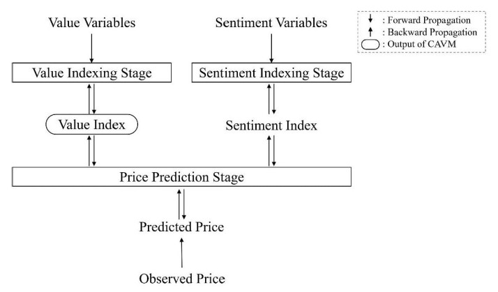
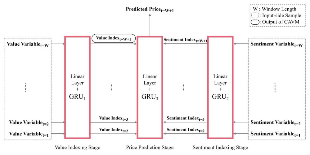
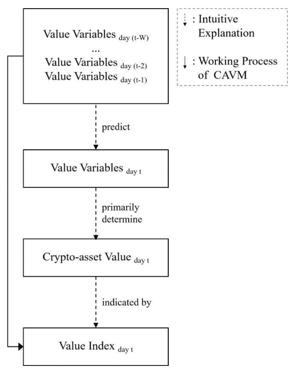
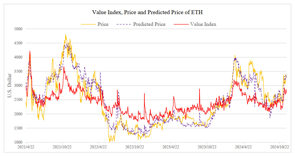
With the rapid expansion of the blockchain ecosystem, crypto asset valuation has become an essential area of study for investors and institutions. Here, we introduce a deep learning framework that was designed to predict the value index of crypto assets by integrating intrinsic value variables and decomposing market prices into value and sentiment components. The Crypto Asset Value-indexing Model (CAVM) was applied to Ethereum's cryptocurrency ETH to demonstrate its effectiveness. Four econometric tests were conducted to verify the informativeness, predictiveness, and reasonability of the generated value indices, as well as the efficiency of price decomposition. Our findings suggested that the value index can serve as a reliable proxy for the intrinsic value of crypto assets, offering a benchmark for investment decisions, consumption, financial reporting, and potential tax implications. Additionally, this research contributes to the literature on asset valuation by proposing a novel method that applies deep learning techniques to intangible assets traded in secondary markets. By utilizing the end-to-end nature and directed acyclic graph structure inherent to deep learning models, we enhance the modeling process with customized loss functions and regularization mechanisms.
Citation: Xi Zhou, Yin Pang, Esther Ying Yang, Jing Rong Goh, Shaun Shuxun Wang. 2025: Valuation of crypto assets on blockchain with deep learning approach, Quantitative Finance and Economics, 9(2): 479-505. doi: 10.3934/QFE.2025016
With the rapid expansion of the blockchain ecosystem, crypto asset valuation has become an essential area of study for investors and institutions. Here, we introduce a deep learning framework that was designed to predict the value index of crypto assets by integrating intrinsic value variables and decomposing market prices into value and sentiment components. The Crypto Asset Value-indexing Model (CAVM) was applied to Ethereum's cryptocurrency ETH to demonstrate its effectiveness. Four econometric tests were conducted to verify the informativeness, predictiveness, and reasonability of the generated value indices, as well as the efficiency of price decomposition. Our findings suggested that the value index can serve as a reliable proxy for the intrinsic value of crypto assets, offering a benchmark for investment decisions, consumption, financial reporting, and potential tax implications. Additionally, this research contributes to the literature on asset valuation by proposing a novel method that applies deep learning techniques to intangible assets traded in secondary markets. By utilizing the end-to-end nature and directed acyclic graph structure inherent to deep learning models, we enhance the modeling process with customized loss functions and regularization mechanisms.

| [1] |
Akyildirim E, Goncu A, Sensoy A (2021) Prediction of cryptocurrency returns using machine learning. Ann Oper Res 297: 3–36. https://doi.org/10.1007/s10479-020-03575-y doi: 10.1007/s10479-020-03575-y

|
| [2] | Ang JS, Ng KW, Chua F (2020) Modeling Time Series Data with Deep Learning: A Review, Analysis, Evaluation and Future Trend. 2020 8th International Conference on Information Technology and Multimedia (ICIMU), 32–37. https://doi.org/10.1109/ICIMU49871.2020.9243546 |
| [3] |
Avramov D, Cheng S, Metzker L (2023) Machine Learning vs. Economic Restrictions: Evidence from Stock Return Predictability. Manage Sci 69: 2587–2619. https://doi.org/10.1287/mnsc.2022.4449 doi: 10.1287/mnsc.2022.4449
|
| [4] |
Bakhtiar T, Luo X, Adelopo I (2023a) Network effects and store-of-value features in the cryptocurrency market. Technol Soc 74: 102320. https://doi.org/10.1016/j.techsoc.2023.102320 doi: 10.1016/j.techsoc.2023.102320
|
| [5] |
Bakhtiar T, Luo X, Adelopo I (2023b) The impact of fundamental factors and sentiments on the valuation of cryptocurrencies. Blockchain-Res Appl 4: 100154. https://doi.org/10.1016/j.bcra.2023.100154 doi: 10.1016/j.bcra.2023.100154
|
| [6] |
Barth JR, Herath HSB, Herath TC, et al. (2020) Cryptocurrency valuation and ethics: a text analytic approach. J Manag Anal 7: 367–388. https://doi.org/10.1080/23270012.2020.1790046 doi: 10.1080/23270012.2020.1790046
|
| [7] |
Biais B, Bisiere C, Bouvard M, et al. (2020) Equilibrium bitcoin pricing. J Financ 78: 967–1014. https://doi.org/10.1111/jofi.13206 doi: 10.1111/jofi.13206
|
| [8] |
Bianchi D, Büchner M, Tamoni A (2021) Bond Risk Premiums with Machine Learning. Rev Financ Stud 34: 1046–1089. https://doi.org/10.1093/rfs/hhaa062 doi: 10.1093/rfs/hhaa062
|
| [9] | Blackwell M (2008) Multiple hypothesis testing: The F-test. Matt Blackwell Res, 1–7. Available from: https://www.mattblackwell.org/files/teaching/ftests.pdf. |
| [10] |
Chen L, Pelger M, Zhu J (2024) Deep Learning in Asset Pricing. Manage Sci 70: 714–750. https://doi.org/10.1287/mnsc.2023.4695 doi: 10.1287/mnsc.2023.4695
|
| [11] | Chung J, Gulcehre C, Cho K, et al. (2014) Empirical evaluation of gated recurrent neural networks on sequence modeling, In: NIPS 2014 Workshop on Deep Learning, December 2014. |
| [12] |
Cong LW, He Z (2019) Blockchain Disruption and Smart Contracts. Rev Financ Stud 32: 1754–1797. https://doi.org/10.1093/rfs/hhz007 doi: 10.1093/rfs/hhz007
|
| [13] |
Cong LW, He Z, Li J (2020) Decentralized Mining in Centralized Pools. Rev Financ Stud 34: 1191–1235. https://doi.org/10.1093/rfs/hhaa040 doi: 10.1093/rfs/hhaa040
|
| [14] |
Costola M, Hinz O, Nofer M, et al. (2023) Machine learning sentiment analysis, COVID-19 news and stock market reactions. Res Int Bus Financ 64: 101881. https://doi.org/10.1016/j.ribaf.2023.101881 doi: 10.1016/j.ribaf.2023.101881
|
| [15] | Dama F, Sinoquet C (2021) Time Series Analysis and Modeling to Forecast: a Survey. Available from: https://arXiv.org/abs/2104.00164 |
| [16] | DiPietro R, Hager GD (2020) Deep learning: RNNs and LSTM, In: Handbook of Medical Image Computing and Computer Assisted Intervention, 503–519, Elsevier. https://doi.org/10.1016/B978-0-12-816176-0.00026-0 |
| [17] |
Dudek G, Fiszeder P, Kobus P, et al. (2024) Forecasting cryptocurrencies volatility using statistical and machine learning methods: A comparative study. Appl Soft Comput 151: 111132. https://doi.org/10.1016/j.asoc.2023.111132 doi: 10.1016/j.asoc.2023.111132
|
| [18] | Fernando S (2021) DVOL-Deribit Implied Volatility Index. Available from: https://insights.deribit.com/exchange-updates/dvol-deribit-implied-volatility-index/. |
| [19] |
García-Monleón F, Danvila-del-Valle I, Lara FJ (2021) Intrinsic value in crypto currencies. Technol Forecast Soc 162: 120393. https://doi.org/10.1016/j.techfore.2020.120393 doi: 10.1016/j.techfore.2020.120393
|
| [20] | Georga EI, Fotiadis DI, Tigas SK (2018) Methodology for Developing a Glucose Prediction Model, In: E. I. Georga, D. I. Fotiadis, & S. K. Tigas (Eds.), Personalized Predictive Modeling in Type 1 Diabetes, 37–59, Academic Press. https://doi.org/10.1016/B978-0-12-804831-3.00003-0 |
| [21] | Goodfellow I, Bengio Y, Courville A (2016) Deep Learning. MIT Press. |
| [22] | Graham B, Dood D (2008) Security Analysis (6th Edition), McGraw Hill. |
| [23] |
Gruber N, Jockisch A (2020) Are GRU Cells More Specific and LSTM Cells More Sensitive in Motive Classification of Text? Front Artif Intell 3: 40. https://doi.org/10.3389/frai.2020.00040 doi: 10.3389/frai.2020.00040
|
| [24] |
Gu S, Kelly B, Xiu D (2020) Empirical Asset Pricing via Machine Learning. Rev Financ Stud 33: 2223–2273. https://doi.org/10.1093/rfs/hhaa009 doi: 10.1093/rfs/hhaa009
|
| [25] | Ioffe S, Szegedy C (2015) Batch normalization: Accelerating deep network training by reducing internal covariate shift. International Conference on Machine Learning. |
| [26] |
Jang H, Lee J (2018) An Empirical Study on Modeling and Prediction of Bitcoin Prices With Bayesian Neural Networks Based on Blockchain Information. IEEE Access 6: 5427–5437. https://doi.org/10.1109/ACCESS.2017.2779181 doi: 10.1109/ACCESS.2017.2779181
|
| [27] | Johnson R, Bufton J, Danie JG (2019) The Valuation of Crypto-assets. Ernst and Young. Available from: https://www.ey.com/en_qa/financial-services--emeia-insights/the-valuation-of-crypto-assets. |
| [28] | Kelly BT, Kuznetsov B, Malamud S, et al. (2025) Artificial Intelligence Asset Pricing Models (January 2025). NBER Working Paper No. w33351. Available from: https://ssrn.com/abstract = 5103546. |
| [29] |
Khan FU, Khan F, Shaikh PA (2023) Forecasting returns volatility of cryptocurrency by applying various deep learning algorithms. Futur Bus J 9: 1–11. https://doi.org/10.1186/s43093-023-00200-9 doi: 10.1186/s43093-023-00200-9
|
| [30] |
Kim HM, Bock GW, Lee G (2021) Predicting Ethereum prices with machine learning based on Blockchain information. Expert Syst Appl 184: 115480. https://doi.org/10.1016/j.eswa.2021.115480 doi: 10.1016/j.eswa.2021.115480
|
| [31] | Kukačka J, Golkov V, Cremers D (2017) Regularization for deep learning: A taxonomy. |
| [32] |
Liebi LJ (2022) Is there a value premium in cryptoasset markets? Econ Model 109: 105777. https://doi.org/10.1016/j.econmod.2022.105777 doi: 10.1016/j.econmod.2022.105777
|
| [33] | Liu Y, Zhang L (2023) Cryptocurrency Valuation: An Explainable AI Approach, In: Arai, K (eds) Intelligent Computing, SAI 2023, Lecture Notes in Networks and Systems, 711, Springer, Cham. https://doi.org/10.1007/978-3-031-37717-4_51 |
| [34] |
Liu Y, Li Z, Ramzi N, Jahangir S (2023) Forecasting cryptocurrency returns with machine learning. Res Int Bus Financ 64: 101905. https://doi.org/10.1016/j.ribaf.2023.101905 doi: 10.1016/j.ribaf.2023.101905
|
| [35] |
Liu Y, Tsyvinski A (2020) Risks and Returns of Cryptocurrency. Rev Financ Stud 34: 2689–2727. https://doi.org/10.1093/rfs/hhaa113 doi: 10.1093/rfs/hhaa113
|
| [36] |
Marty T, Vanstone B, Hahn T (2020) News media analytics in finance: a survey. Account Financ 60: 1385–1434. https://doi.org/10.1111/acfi.12466 doi: 10.1111/acfi.12466
|
| [37] |
Naeem MA, Mbarki I, Shahzad SJ (2021) Predictive role of online investor sentiment for cryptocurrency market: Evidence from happiness and fears. Int Rev Econ Financ 73: 496–514. https://doi.org/10.1016/j.iref.2021.01.008 doi: 10.1016/j.iref.2021.01.008
|
| [38] | Pagnotta ES, Buraschi A (2018) An Equilibrium Valuation of Bitcoin and Decentralized Network Assets. SSRN Electron J. https://doi.org/10.2139/ssrn.3142022 |
| [39] |
Poyser O (2019) Exploring the dynamics of Bitcoin's price: a Bayesian structural time series approach. Eur Econ Rev 9: 29–60. https://doi.org/10.1007/s40822-018-0108-2 doi: 10.1007/s40822-018-0108-2
|
| [40] |
Saad M, Choi J, Nyang D, et al. (2020) Toward Characterizing Blockchain-Based Cryptocurrencies for Highly Accurate Predictions. IEEE Syst J 14: 321–332. https://doi.org/10.1109/JSYST.2019.2927707 doi: 10.1109/JSYST.2019.2927707
|
| [41] |
Schilling L, Uhlig H (2019) Some simple bitcoin economics. J Monetary Econ 106: 16–26. https://doi.org/10.1016/j.jmoneco.2019.07.002 doi: 10.1016/j.jmoneco.2019.07.002
|
| [42] | Shapiro C, Varian H (1999) Information Rules: A Strategic Guide to The Network Economy, Harvard Business School Press, 1999. |
| [43] |
Sockin M, Xiong W (2020) A Model of Cryptocurrencies. Manage Sci 69: 6684–6707. https://doi.org/10.3386/w26816 doi: 10.3386/w26816
|
| [44] |
Thies F, Wallbach S, Wessel M, et al. (2022) Initial coin offerings and the cryptocurrency hype - the moderating role of exogenous and endogenous signals. Electron Mark 32: 1691–1705. https://doi.org/10.1007/s12525-021-00460-9 doi: 10.1007/s12525-021-00460-9
|
| [45] |
Valencia F, Gómez-Espinosa A, Valdés-Aguirre B (2019) Price Movement Prediction of Cryptocurrencies Using Sentiment Analysis and Machine Learning. Entropy 21: 589. https://doi.org/10.3390/e21060589 doi: 10.3390/e21060589
|
| [46] | Verma A, Walia R, Kumar V (2024) Advanced predictive analytics for cryptocurrency valuation: A comparative study of machine learning and deep learning approaches, In: Computational Methods in Science and Technology, 1st Edition, CRC Press. https://doi.org/10.1201/9781003501244-60 |
| [47] |
Wan X, Yang J, Marinov S, et al. (2021) Sentiment correlation in financial news networks and associated market movements. Sci Rep 11: 3062. https://doi.org/10.1038/s41598-021-82338-6 doi: 10.1038/s41598-021-82338-6
|
| [48] |
Xing FZ, Cambria E, Welsch RE (2018): Natural language based financial forecasting: a survey. Artif Intell Rev 50: 49–73. https://doi.org/10.1007/s10462-017-9588-9 doi: 10.1007/s10462-017-9588-9
|
| [49] |
Yildirim H, Bekun FV (2023) Predicting volatility of bitcoin returns with ARCH, GARCH and EGARCH models. Future Bus J 9: 75. https://doi.org/10.1186/s43093-023-00255-8 doi: 10.1186/s43093-023-00255-8
|
| [50] |
Zhang W, Wang P (2020) Investor attention and the pricing of cryptocurrency market. Evol Inst Econ Rev 17: 445–468. https://doi.org/10.1007/s40844-020-00182-1 doi: 10.1007/s40844-020-00182-1
|
 QFE-09-02-016-s001.pdf QFE-09-02-016-s001.pdf |
 |
Figures(4) / Tables(8)

Xi Zhou, Yin Pang, Esther Ying Yang, Jing Rong Goh, Shaun Shuxun Wang. 2025: Valuation of crypto assets on blockchain with deep learning approach, Quantitative Finance and Economics, 9(2): 479-505. doi: 10.3934/QFE.2025016


 DownLoad: