In this paper, we investigate a retrial tandem queueing system with a finite number of queues. Each queue consists of a finite buffer and a single server with phase-type distributed service times. Customers arrive at the system according to a Markovian arrival process (MAP). At any queue, a customer that finds both the server busy and the buffer full enters a common orbit and makes repeated attempts to rejoin the first queue after exponentially distributed time intervals. This system models telecommunication networks with linear topology that implement retransmission protocols for lost data packets. We provide a complete mathematical analysis for the two-queue system with an infinite-capacity orbit, deriving the ergodicity condition, stationary state distribution, and key performance characteristics. For systems with an arbitrary number of queues, we develop a comprehensive solution approach that combines queueing theory methods, discrete-event simulation, and machine learning techniques to predict the mean sojourn time. We implement and compare multiple machine learning methods, evaluating their predictive performance through extensive numerical experiments.
Citation: Vladimir Vishnevsky, Valentina Klimenok, Olga Semenova, Minh Cong Dang. Retrial tandem queueing system with correlated arrivals[J]. AIMS Mathematics, 2025, 10(5): 10650-10674. doi: 10.3934/math.2025485
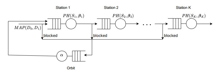
In this paper, we investigate a retrial tandem queueing system with a finite number of queues. Each queue consists of a finite buffer and a single server with phase-type distributed service times. Customers arrive at the system according to a Markovian arrival process (MAP). At any queue, a customer that finds both the server busy and the buffer full enters a common orbit and makes repeated attempts to rejoin the first queue after exponentially distributed time intervals. This system models telecommunication networks with linear topology that implement retransmission protocols for lost data packets. We provide a complete mathematical analysis for the two-queue system with an infinite-capacity orbit, deriving the ergodicity condition, stationary state distribution, and key performance characteristics. For systems with an arbitrary number of queues, we develop a comprehensive solution approach that combines queueing theory methods, discrete-event simulation, and machine learning techniques to predict the mean sojourn time. We implement and compare multiple machine learning methods, evaluating their predictive performance through extensive numerical experiments.

| [1] |
A. Heindl, K. Mitchell, A. van de Liefvoort, Correlation bounds for second order MAPs with application to queueing network decomposition, Perform. Eval., 63 (2006), 533–577. http://doi.org/10.1016/j.peva.2005.06.003 doi: 10.1016/j.peva.2005.06.003

|
| [2] | S. Balsamo, Queueing networks with blocking: Analysis, solution algorithms and properties, In: Lecture Notes in Computer Science, Berlin: Springer, 5233 (2011), 233–257. http://doi.org/10.1007/978-3-642-02742-0_11 |
| [3] | B. W. Gnedenko, D. Konig, Handbuch der bedienungstheorie, Berlin: Akademie Verlag, 1983. |
| [4] |
M. F. Neuts, A versatile Markovian point process, J. Appl. Prob., 16 (1979), 764–779. http://doi.org/10.2307/3213143 doi: 10.2307/3213143
|
| [5] |
D. M. Lucantoni, New results on the single server queue with a batch markovian arrival process, Commun. Stat. Stoch. Models, 7 (1991), 1–46. http://doi.org/10.1080/15326349108807174 doi: 10.1080/15326349108807174
|
| [6] |
S. A. Dudin, A. N. Dudin, O. S. Dudina, S. R. Chakravarthy, Analysis of a tandem queuing system with blocking and group service in the second node, Int. J. Syst. Sci. Oper. Log., 10 (2023), 2235270. http://doi.org/10.1080/23302674.2023.2235270 doi: 10.1080/23302674.2023.2235270
|
| [7] |
Z. Lian, L. Liu, A tandem network with MAP inputs, Oper. Res. Lett., 36 (2008), 189–195. http://doi.org/10.1016/j.orl.2007.04.004 doi: 10.1016/j.orl.2007.04.004
|
| [8] |
A. Gomez-Corral, A tandem queue with blocking and Markovian arrival process, Queueing Syst., 41 (2002), 343–370. http://doi.org/10.1023/A:1016235415066 doi: 10.1023/A:1016235415066
|
| [9] |
C. Kim, A. Dudin, V. Klimenok, O. Taramin, A Tandem BMAP/G/1 → •/M/N/0 queue with group occupation of servers at the second station, Math. Prob. Eng., 2012 (2012), 324604. http://doi.org/10.1155/2012/324604 doi: 10.1155/2012/324604
|
| [10] |
C. Kim, S. Dudin, Priority tandem queueing model with admission control, Comput. Indust. Eng., 61 (2011), 131–140. http://doi.org/10.1016/j.cie.2011.03.003 doi: 10.1016/j.cie.2011.03.003
|
| [11] |
B. K. Kumar, R. Sankar, R. N. Krishnan, R. Rukmani, Performance analysis of multi-processor two-stage tandem call center retrial queues with non-reliable processors, Methodol. Comput. Appl. Probab., 24 (2022), 95–142. http://doi.org/10.1007/s11009-020-09842-6 doi: 10.1007/s11009-020-09842-6
|
| [12] |
A. Dudin, A. Nazarov, On a tandem queue with retrials and losses and state dependent arrival, service and retrial rates, Int. J. Oper. Res., 29 (2017), 170–182. http://doi.org/10.1504/IJOR.2017.083954 doi: 10.1504/IJOR.2017.083954
|
| [13] | C. Kim, A. Dudin, V. Klimenok, Tandem retrial queueing system with correlated arrival flow and operation of the second station described by a Markov chain, In: Computer Networks: 19th International Conference, CN 2012, Szczyrk, Poland, 291 (2012), 370–382. http://doi.org/10.1007/978-3-642-31217-5_39 |
| [14] |
C. S. Kim, V. Klimenok, O. Taramin, A tandem retrial queueing system with two Markovian flows and reservation of channels, Comput. Oper. Res, , 37 (2010), 1238–1246. http://doi.org/10.1016/j.cor.2009.03.030 doi: 10.1016/j.cor.2009.03.030
|
| [15] |
C. S. Kim, S. H. Park, A. Dudin, V. Klimenok, G. V. Tsarenkov, Investigaton of the BMAP/G/1 → •/PH/1/M tandem queue with retrials and losses, Appl. Math. Model., 34 (2010), 2926–2940. http://doi.org/10.1016/j.apm.2010.01.003 doi: 10.1016/j.apm.2010.01.003
|
| [16] |
A. N. Dudin, R. Manzo, R. Piscopo, Single server retrial queue with group admission of customers, Comput. Oper. Res., 61 (2015), 89–99. https://doi.org/10.1016/j.cor.2015.03.008 doi: 10.1016/j.cor.2015.03.008
|
| [17] | G. Falin, J. G. C. Templeton, Retrial queues, Florida: CRC Press, 1997. |
| [18] | J. R. Artalejo, A. Gomez-Corral, Retrial queueing systems, Berlin: Springer, 2008. |
| [19] |
V. Klimenok, O. Dudina, Retrial tandem queue with controllable strategy of repeated attempts, Qual. Technol. Quant. Manag., 14 (2016), 74–93. http://doi.org/10.1080/16843703.2016.1189177 doi: 10.1080/16843703.2016.1189177
|
| [20] |
C. S. Kim, V. Klimenok, A. Dudin, Priority tandem queueing system with retrials and reservation of channels as a model of call center, Comput. Indust. Eng., 96 (2016), 61–71. http://doi.org/10.1016/j.cie.2016.03.012 doi: 10.1016/j.cie.2016.03.012
|
| [21] |
S. Dudin, A. Dudin, R. Manzo, L. Rarità, Analysis of semi-open queueing network with correlated arrival process and multi-server nodes, Oper. Res. Forum, 5 (2024), 99. https://doi.org/10.1007/s43069-024-00383-z doi: 10.1007/s43069-024-00383-z
|
| [22] |
K. Avrachenkov, U. Yechiali, On tandem blocking queues with a common retrial queue, Comput. Oper. Res., 37 (2010), 1174–1180. http://doi.org/10.1016/j.cor.2009.10.004 doi: 10.1016/j.cor.2009.10.004
|
| [23] | S. V. Paul, A. A. Nazarov, T. Phung-Duc, M. Morozova, Mathematical model of the tandem retrial queue M/GI/1/M/1 with a common orbit, In: Communications in Computer and Information Science, Berlin: Springer, 1605 (2022), 131–143. http://doi.org/10.1007/978-3-031-09331-9_11 |
| [24] | A. A. Nazarov, S. V. Paul, T. Phung-Duc, M. Morozova, Analysis of tandem retrial queue with common orbit and MMPP incoming flow, In: Lecture Notes Comput. Sci., Berlin: Springer, 13766 (2023), 270–283. http://doi.org/10.1007/978-3-031-23207-7_21 |
| [25] | V. M. Vishnevsky, A. N. Dudin, D. V. Kozyrev, A. A. Larionov, Methods of performance evaluation of broadband wireless networks along the long transport routes, In: Distributed Computer and Communication Networks. DCCN 2015. Communications in Computer and Information Science, Spinger, 601 (2016), 72–85. http://doi.org/10.1007/978-3-319-30843-2_8 |
| [26] | V. M. Vishnevsky, A. V. Gorbunova, Application of machine learning methods to solving problems of queuing theory, In: International Conference on Information Technologies and Mathematical Modelling, Springer, 1605 (2022), 304–316. http://doi.org/10.1007/978-3-031-09331-9_24 |
| [27] |
V. Vishnevsky, V. Klimenok, A. Solokov, A. Larionov, Performance evaluation of the priority multi-server system MMAP/PH/M/N using machine learning methods, Mathematics, 9 (2021), 3236. http://doi.org/10.3390/math9243236 doi: 10.3390/math9243236
|
| [28] |
V. Vishnevsky, V. Klimenok, A. Solokov, A. Larionov, Investigation of the fork-join system with markovian arrival process arrivals and phase-type service time distribution using machine learning methods, Mathematics, 12 (2024), 0659. http://doi.org/10.3390/math12050659 doi: 10.3390/math12050659
|
| [29] | V. M. Vishnevsky, A. A. Larionov, A. A. Mukhtarov, A. M. Sokolov, Investigation of tandem queueing systems using machine learning methods, Control Sci., 4 (2024), 10–21. |
| [30] | A. N. Dudin, V. I. Klimenok, V. M. Vishnevsky, The theory of queuing systems with correlated flows, Switzerland: Springer, 2020. http://doi.org/10.1007/978-3-030-32072-0 |
| [31] | M. F. Neuts, Structured stochastic matrices of M/G/1 type and their applications, New York: Marcel Dekker, 1989. |
| [32] |
V. Klimenok, A. Dudin, Multi-dimensional asymptotically quasi-Toeplitz Markov chains and their application in queueing theory, Queueing Syst., 54 (2006), 245–259. http://doi.org/10.1007/s11134-006-0300-z doi: 10.1007/s11134-006-0300-z
|
| [33] | F. Gantmakher, The matrix theory, Moscow: Science, 1967. |
| [34] | M. C. Dang, Prediction of a multiphase queuing system performance using machine learning method, in Russian, Trudy MFTI, 16 (2024), 37–45. |
| [35] | V. Vishnevsky, A. Larionov, I. Roman, O. Semenova, Estimation of IEEE 802.11 DCF access performance in wireless networks with linear topology using PH service time approximations and MAP input, In: IEEE 11th Int. Conf. on Application of Information and Communication Technologies, 2017. http://doi.org/10.1109/ICAICT.2017.8687247 |
| [36] | V. N. Vapnik, The nature of statistical learning theory, New York: Springer, 2000. |
| [37] |
R. E. Schapire, The strength of weak learnability, Mach. Learn., 5 (1990), 245–259. http://doi.org/10.1007/BF00116037 doi: 10.1007/BF00116037
|
| [38] | Y. Liu, J. Zhang, C. Gao, J. Qu, L. Ji, Natural-logarithm-rectified activation function in convolutional neural networks, 2019 IEEE 5th International Conference on Computer and Communications, 2019, 2000–2008. http://doi.org/10.1109/ICCC47050.2019.9064398 |


Figures(5) / Tables(10)

Vladimir Vishnevsky, Valentina Klimenok, Olga Semenova, Minh Cong Dang. Retrial tandem queueing system with correlated arrivals[J]. AIMS Mathematics, 2025, 10(5): 10650-10674. doi: 10.3934/math.2025485


 DownLoad: