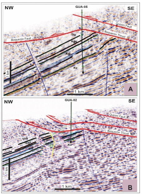
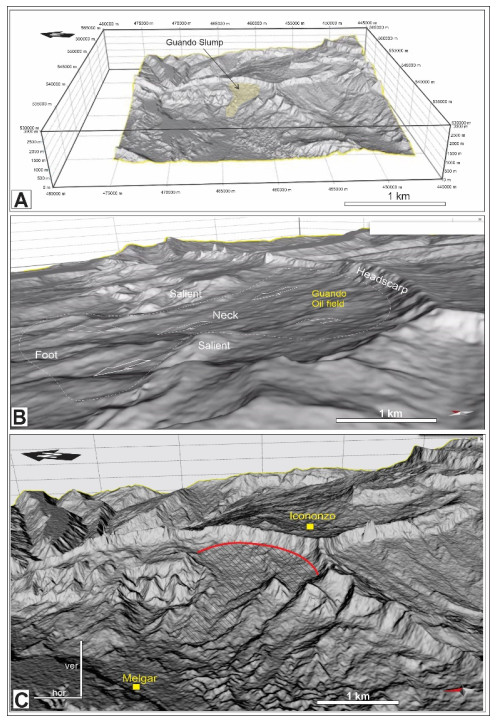
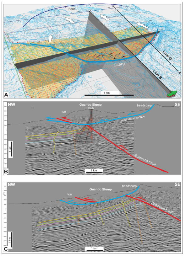
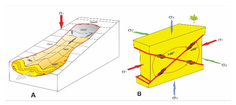
A detailed geological study of the Guando oilfield has identified a modern landslide phenomenon that significantly alters the previous structural model and affects production challenges. The multi-compositional nature of the oil-bearing Cretaceous sequences of the Villeta Group, the rugged relief, the climatic incidence, and seismic activity in the Upper Magdalena Valley trigger the Guando Slump, which adjusts the topography to levels of greater stability. The previous tectonic model of the Guando oilfield was based on the superposition of an internally disturbed block by the Boquerón thrust. However, in its westernmost segment, this structure shows angular incompatibilities with the expected horizontal stress fields. Therefore, based on a detailed 3D interpretation of geological maps, DEM, and available geophysical data, we propose that this segment must be associated with the surface of the underlying detachment of the Guando Slump. The horizontal displacement of the landslide, ranging from 1 to 2 km, deforms and collapses the wells that reach the underlying productive reservoirs. This study describes the relationship of this new tectonic model of the Guando oilfield, considering the westernmost segment of the Boquerón thrust as a detachment of the Guando Slump. This real-life example, if properly monitored, will contribute to a better management of the possible causes and consequences of technical problems encountered in the Guando oilfield exploration and prevent catastrophic risks to the production facilities.
Citation: Eduardo Antonio Rossello. Effects of the Guando Slump on the tectonic interpretation of the Boquerón Thrust in the Guando oilfield [Tolima, Colombia][J]. AIMS Geosciences, 2025, 11(2): 370-386. doi: 10.3934/geosci.2025016
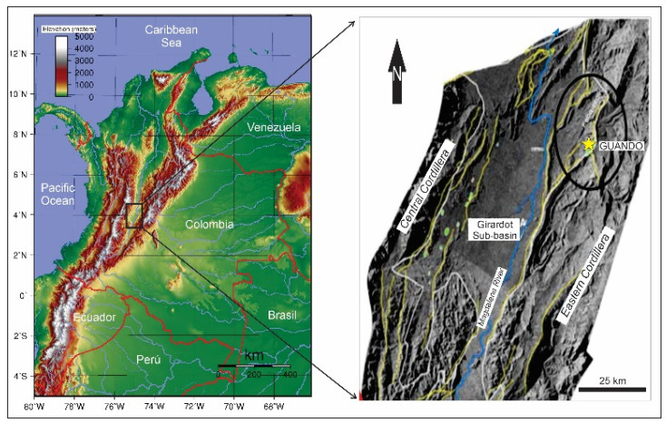
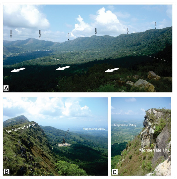
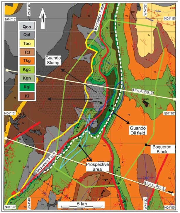
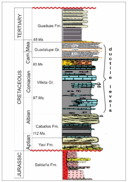
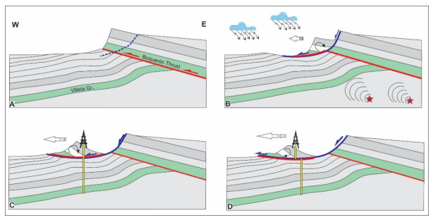
A detailed geological study of the Guando oilfield has identified a modern landslide phenomenon that significantly alters the previous structural model and affects production challenges. The multi-compositional nature of the oil-bearing Cretaceous sequences of the Villeta Group, the rugged relief, the climatic incidence, and seismic activity in the Upper Magdalena Valley trigger the Guando Slump, which adjusts the topography to levels of greater stability. The previous tectonic model of the Guando oilfield was based on the superposition of an internally disturbed block by the Boquerón thrust. However, in its westernmost segment, this structure shows angular incompatibilities with the expected horizontal stress fields. Therefore, based on a detailed 3D interpretation of geological maps, DEM, and available geophysical data, we propose that this segment must be associated with the surface of the underlying detachment of the Guando Slump. The horizontal displacement of the landslide, ranging from 1 to 2 km, deforms and collapses the wells that reach the underlying productive reservoirs. This study describes the relationship of this new tectonic model of the Guando oilfield, considering the westernmost segment of the Boquerón thrust as a detachment of the Guando Slump. This real-life example, if properly monitored, will contribute to a better management of the possible causes and consequences of technical problems encountered in the Guando oilfield exploration and prevent catastrophic risks to the production facilities.

| [1] | Buitrago J (1994) Petroleum systems of the Neiva Area, Upper Magdalena Valley, Colombia. In: Magoon LB, WG Dow (eds.), The Petroleum System – from source to trap. AAPG, Memoir 60: 483–497. https://doi.org/10.1306/M60585C30 |
| [2] | Mojica J, Franco R (1990) Estructura y evolución tectónica del Valle Medio y Superior del Magdalena, Colombia. Geol Colombiana 17: 41–64. |
| [3] | Rincón G, Garzón JC, de Moraes JJ (2003) Campo Guando, Primer Descubrimiento de la Antesala del Siglo XXI en el Valle Superior del Magdalena, Colombia. 8th Simposio Bolivariano - Exploración Petrolera en las Cuencas Subandinas. Cartagena, Colombia. https://www.earthdoc.org/content/papers/10.3997/2214-4609-pdb.33.Paper66 |
| [4] |
Sarmiento LF, Rangel A (2004) Petroleum systems of the Upper Magdalena Valley, Colombia. Mar Petrol Geol 21: 373–391. https://doi.org/10.1016/j.marpetgeo.2003.11.019 doi: 10.1016/j.marpetgeo.2003.11.019

|
| [5] |
Ramón J, Rosero A (2006) Multiphase structural evolution of the western margin of the Girardot Subbasin, Upper Magdalena Valley, Colombia. J S Am Earth Sci 21: 493–509. https://doi.org/10.1016/j.jsames.2006.07.012 doi: 10.1016/j.jsames.2006.07.012
|
| [6] | Barrero D, Pardo A, Vargas CA, et al. (2007) Colombian sedimentary basins: nomenclature, boundaries and petroleum geology, a new proposal. Agencia Nacional de Hidrocarburos - B&M Exploration Ltda. 35pp. Bogotá. |
| [7] | Roncancio J, Martínez M (2011) Upper Magdalena Basin. In: Cediel F, Colmenares F (eds.), Petroleum Geology of Colombia. Fondo Editorial Universidad Eafit, vol. 14: 183 pp. Medellin. |
| [8] |
Rossello EA, Saavedra JL (2020) El deslizamiento gravitatorio de Guando (Tolima, Colombia): características morfoestructurales y consecuencias de su interpretación. Bol Geol 42: 151–170. https://doi.org/10.18273/revbol.v42n3-2020007 doi: 10.18273/revbol.v42n3-2020007
|
| [9] | Arévalo-Chaves DA, Parias-Villalba JP (2013) Análisis de amenaza por fenómenos de remoción en masa en la región del Boquerón ubicada entre los departamentos de Cundinamarca y Tolima mediante el uso de un Sistema de información geográfica de libre distribución. Tesis, Universidad Católica de Colombia, Bogotá, Colombia, 73. |
| [10] |
Pfiffner OA (2017) Thick-skinned and thin-skinned tectonics: A global perspective. Geosciences 7: 1–89. https://doi.org/10.3390/geosciences7030071 doi: 10.3390/geosciences7030071
|
| [11] |
Nemčok A, Pašek J, Rybář J (1972) Classification of landslides and other mass movements. Rock Mechanics 4: 71–78. https://doi.org/10.1007/BF01239137 doi: 10.1007/BF01239137
|
| [12] |
Hutchinson JN, Bhandari RK (1971) Undrained loading, a fundamental mechanism of mudflows and other mass movements. Géotechnique 21: 353–358. https://doi.org/10.1680/geot.1971.21.4.353 doi: 10.1680/geot.1971.21.4.353
|
| [13] | Varnes DJ (1978) Slope movement types and processes. In: Schuster RL, Krizek RJ (eds.), Landslides, analysis and control. Transportation research board, National Academy of Sciences. Special report 176: Chapter 2: 11–33. https://trid.trb.org/view/86168 |
| [14] | Crozier MJ (1986) Landslides: causes, consequences and environment. Croom Helm. 252. London, https://doi.org/10.1080/03036758.1988.10429158 |
| [15] | Cruden DM, Varnes DJ (1996) Landslide types and processes. In: Turner AK, Schuster RL (eds.), Landslides investigation and mitigation. US National Research Council. Special Report 247, Chapter 3: 36–75. |
| [16] | Dikau R, Brunsdsen D, Schrott L, et al. (1996) Landslides recognition: identification, movement and causes. John Wiley & Sons. 274. |
| [17] | Leroueil S, Locat J, Vaunat J, et al. (1996) Geotechnical characterization of slope movements. In: Senneset K (ed.), Landslides. Balkema, Rotterdam 1: 53–74. |
| [18] | Sassa K (1999) Introduction. In: Sassa K (ed.), Landslides of the world. Kyoto University Press. 3–18. https://doi.org/10.1007/3-540-27129-5_5 |
| [19] |
Alcántara-Ayala I (2000) Landslides: ¿deslizamientos o movimientos del terreno? Definición, clasificaciones y terminología. Investigaciones Geográficas: Boletín – Instituto de Geografía, Universidad Nacional Autónoma de México, 41: 7–25. https://doi.org/10.14350/rig.59101 doi: 10.14350/rig.59101
|
| [20] |
Alsop GI, Marco S, Weinberger R, et al. (2017) Upslope-verging back thrusts developed during downslope-directed slumping of mass transport deposits. J Struct Geol 100: 45–61. https://doi.org/10.1016/j.jsg.2017.05.006 doi: 10.1016/j.jsg.2017.05.006
|
| [21] | Easterbrook DJ (1993) Surfaces processes and landforms. 2nd Ed. Prentice Hall. Nueva York, 230. |
| [22] | Glade T, Anderson M, Crozier MJ (2012) Landslide hazard and risk. John Wiley & Sons. Chichester, 807. https://doi.org/10.1002/9780470012659 |
| [23] | Ng KS, Chew YM (2019) Slope stability analysis of embankment over stone column improved ground. J Eng Sci Technol 14: 3582–3596. |
| [24] |
Hennings P, Olson J, Thompson L (2000) Combining outcrop data and three-dimensional structural models to characterize fracture reservoirs: an example from Wyoming. AAPG Bulletin 84: 830–849. https://doi.org/10.1306/A967340A-1738-11D7-8645000102C1865D doi: 10.1306/A967340A-1738-11D7-8645000102C1865D
|
| [25] |
Hergarten S, Robl J, Stüwe K (2014) Extracting topographic swath profiles across curved geomorphic features. Earth Surf Dynam 2: 97–104. https://doi.org/10.5194/esurf-2-97-2014 doi: 10.5194/esurf-2-97-2014
|
| [26] |
Jaimes E, De Freitas M (2006) An Albian-Cenomanian unconformity in the Northern Andes: Evidence and tectonic significance. J S Am Earth Sci 21: 466–492. https://doi.org/10.1016/j.jsames.2006.07.011 doi: 10.1016/j.jsames.2006.07.011
|
| [27] |
Mantilla M, Salazar CC, Rossello EA (2024) The geology of the La Hocha High and its associated oil fields (southern Upper Magdalena Valley, Colombia): a new 3D structural model based on 3D subsurface data. Geociências 43: 537–557. https://doi.org/10.5016/geociencias.v43i4.18579 doi: 10.5016/geociencias.v43i4.18579
|
| [28] |
Cediel F, Mojica J, Macía C (1981) Definición estratigráfica del Triásico de Colombia, Suramérica. Las Formaciones Luisa, Payandé, Saldaña. Sus columnas estratigráficas. Newsl Stratigr 9: 73–104. https://doi.org/10.1127/nos/9/1980/73 doi: 10.1127/nos/9/1980/73
|
| [29] | Horton BK, Parra M, Mora A (2020) Construction of the Eastern Cordillera of Colombia: Insights from the sedimentary record. In: Gómez J, Mateus-Zabala D (eds.), The Geology of Colombia, Volume 3 Paleogene – Neogene. Servicio Geológico Colombiano, Publicaciones Geológicas Especiales 37: 67–88. Bogotá. https://doi.org/10.32685/pub.esp.37.2019.03 |
| [30] |
Cobbold PR, Davy P, Gapais D, et al. (1993) Sedimentary basins and crustal thickening. Sediment Geol 86: 77–89. https://doi.org/10.1016/0037-0738(93)90134-Q doi: 10.1016/0037-0738(93)90134-Q
|
| [31] | Schamel S (1991) Middle and Upper Magdalena Basins, Colombia. In: Biddle KT (ed.), Active margin basin. AAPG, Memoir, 52. Chapter 10: 283–301. https://doi.org/10.1306/M52531C10 |
| [32] |
Cooper MA, Addison FT, Alvarez R, et al. (1995) Basin development and tectonic history of the Llanos Basin, Eastern Cordillera and Magdalena Valley, Colombia. AAPG Bulletin 79: 1421–1443. https://doi.org/10.1306/7834D9F4-1721-11D7-8645000102C1865D doi: 10.1306/7834D9F4-1721-11D7-8645000102C1865D
|
| [33] | Toro J, Roure F, Bordas-Le Floch N, et al. (2004) Thermal and kinematic evolution of the Eastern Cordillera fold and thrust belt, Colombia. In: Swennen R et al. (eds.), Deformation, fluid flow, and reservoir appraisal in foreland fold and thrust belts. AAPG, Hedberg Series, 1: 79–115. https://doi.org/10.1306/1025687H13114 |
| [34] |
Sarmiento-Rojas LF, Van Wess JD, Cloetingh S (2006) Mesozoic transtensional basin history of the Eastern Cordillera, Colombian Andes: Inferences from tectonic models. J S Am Earth Sci 21: 383–411. https://doi.org/10.1016/j.jsames.2006.07.003 doi: 10.1016/j.jsames.2006.07.003
|
| [35] |
Mora-Páez H, Mencin, DJ, Molnar P, et al. (2016) GPS velocities and the construction of the Eastern Cordillera of the Colombian Andes. Geophys Res Lett 43: 8407–8416. http://doi.org/10.1002/2016GL069795 doi: 10.1002/2016GL069795
|
| [36] |
Rossello EA, Gallardo A (2022) The Sierra Nevada de Santa Marta (Colombia) and Nevado de Famatina (Argentina) positive syntaxes: two comparable exceptional relieves in the Andes foreland. J Struct Geol 160: https://doi.org/10.1016/j.jsg.2022.104618 doi: 10.1016/j.jsg.2022.104618
|
| [37] |
Cobbold PR, Rossello EA, Roperch P, et al. (2007) Distribution, timing, and causes of Andean deformation across South America. Geological Society, London, Special Publications 272: 321–343. https://doi.org/10.1144/GSL.SP.2007.272.01.17 doi: 10.1144/GSL.SP.2007.272.01.17
|
| [38] |
Lewis KB (1971) Slumping on a continental slope inclined at 1–4°. Sedimentology 16: 97–110. http://doi.org/10.1111/j.1365-3091.1971.tb00221.x doi: 10.1111/j.1365-3091.1971.tb00221.x
|
| [39] | Martinsen OJ (1994) Mass movements. In: Maltman A (ed.), The geological deformation of sediments. Chapman & Hall, London, 27–165. http://doi.org/10.1007/978-94-011-0731-0_5 |
| [40] |
Bull S, Cartwright J, Huuse M (2009) A review of kinematic indicators from mass-transport complexes using 3D seismic data. Mar Petrol Geol 26: 1132–1151. http://doi:10.1016/j.marpetgeo.2008.09.011 doi: 10.1016/j.marpetgeo.2008.09.011
|
| [41] |
Sobiesiak MS, Kneller B, Alsop GI, et al. (2018) Styles of basal interaction beneath mass transport deposits. Mar Petrol Geol 98: 629–639. http://doi.org/10.1016/j.marpetgeo.2018.08.028 doi: 10.1016/j.marpetgeo.2018.08.028
|
| [42] |
Rossello EA, López-Isaza JA (2023) The structural control of mineralizations by dilatancies due to differential thermal expansivity (in disseminated deposits) and faults bending (in veins): revision and working hypothesis. Rev Mex Cienc Geol 40: 16–34. http://dx.doi.org/10.22201/cgeo.20072902e.2023.1.1716 doi: 10.22201/cgeo.20072902e.2023.1.1716
|
| [43] | Gostelow TP (1991) Rainfall and landslides. In: Almeida-Teixeira F et al. (eds.), Prevention and control of landslides and other mass movements. Commission of the European Communities. Report EUR 12918: 139–161. |
| [44] | Girty GH (2009) Perilous Earth: Understanding processes behind natural disasters. Chapter 7, 1–17, Montezuma Publishing, San Diego. Available from: https://studylib.net/doc/8423341/chapter-1. |
| [45] |
Hungr O, Leroueil S, Picarelli L (2013) The Varnes classification of landslide types, an update. Landslides 11: 167–194. https://doi.org/10.1007/s10346-013-0436-y doi: 10.1007/s10346-013-0436-y
|
| [46] | Ramsay JG, Huber MI (1983) The techniques of modern structural geology: strain analyses. Academic Press. 393. |
| [47] | Price NJ, Cosgrove JW (1990) Analysis of geological structures. Cambridge University Press. 502. |
| [48] |
Working Party for World Landslide Inventory (1995) A suggested method for describing the rate of movement of a landslide. Bulletin of the International Association of Engineering Geology 52: 75–78. https://doi.org/10.1007/BF02639593 doi: 10.1007/BF02639593
|
| [49] |
Tofani V, Raspini F, Catani F, et al. (2013) Persistent Scatterer Interferometry (PSI) technique for landslide characterization and monitoring. Remote Sens 5: 1045–1065. https://doi.org/10.3390/rs5031045 doi: 10.3390/rs5031045
|
| [50] |
Tiampo KF, González PJ, Samsonov SS (2013) Results for aseismic creep on the Hayward fault using polarization persistent scatterer InSAR. Earth Planet Sc Lett 367: 157–165. https://doi.org/10.1016/j.epsl.2013.02.019 doi: 10.1016/j.epsl.2013.02.019
|
| [51] | Záruba Q, Mencl V (1969) Landslides and their control. Elsevier. Amsterdam, 270. |
| [52] | Schuster RL, Salcedo DA, Valenzuela L (2002) Overview of catastrophic landslides of South America in the twentieth century. In: Evans SG, DeGraff JV (eds.). Catastrophic Landslides: effects, occurrence, and mechanisms The Geological Society of America. Reviews in Engineering Geology, XV: 1–34. https://doi.org/10.1130/REG15-p1 |
Figures(9)

Eduardo Antonio Rossello. Effects of the Guando Slump on the tectonic interpretation of the Boquerón Thrust in the Guando oilfield [Tolima, Colombia][J]. AIMS Geosciences, 2025, 11(2): 370-386. doi: 10.3934/geosci.2025016


 DownLoad: