Sales forecasting is very important in retail management. It helps with decisions about inventory, staffing, and planning promotions. In this study, we looked at how to balance the accuracy of predictions with how easy it is to understand the machine learning models used in sales forecasting. We used public data from Rossmann stores to study various factors like promotions, holidays, and store features that affect daily sales. We compared a complex, highly accurate model (XGBoost) with simpler, easier-to-understand linear regression models. To find a middle ground, we created a hybrid model called LR_XGBoost. This model changes a linear regression model to match the predictions of XGBoost. The hybrid model keeps the strong predictive power of complex models but makes the results easier to understand, which is important for making decisions in retail. Our study shows that our hybrid model offers a good balance, providing reliable sales forecasts with more transparency than standard linear regression. This makes it a valuable tool for retail managers who need accurate forecasts and a clear understanding of what influences sales. The model's consistent performance across datasets also suggests it can be used in various retail settings to improve efficiency and help with strategic decisions.
Citation: Miguel Arantes, Wenceslao González-Manteiga, Javier Torres, Alberto Pinto. Striking a balance: navigating the trade-offs between predictive accuracy and interpretability in machine learning models[J]. Electronic Research Archive, 2025, 33(4): 2092-2117. doi: 10.3934/era.2025092
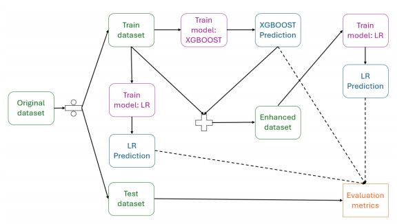
Sales forecasting is very important in retail management. It helps with decisions about inventory, staffing, and planning promotions. In this study, we looked at how to balance the accuracy of predictions with how easy it is to understand the machine learning models used in sales forecasting. We used public data from Rossmann stores to study various factors like promotions, holidays, and store features that affect daily sales. We compared a complex, highly accurate model (XGBoost) with simpler, easier-to-understand linear regression models. To find a middle ground, we created a hybrid model called LR_XGBoost. This model changes a linear regression model to match the predictions of XGBoost. The hybrid model keeps the strong predictive power of complex models but makes the results easier to understand, which is important for making decisions in retail. Our study shows that our hybrid model offers a good balance, providing reliable sales forecasts with more transparency than standard linear regression. This makes it a valuable tool for retail managers who need accurate forecasts and a clear understanding of what influences sales. The model's consistent performance across datasets also suggests it can be used in various retail settings to improve efficiency and help with strategic decisions.

| [1] |
S. Hochreiter, J. Schmidhuber, Long short-term memory, Neural Comput., 9 (1997), 1735–1780. http://dx.doi.org/10.1162/neco.1997.9.8.1735 doi: 10.1162/neco.1997.9.8.1735

|
| [2] |
R. Roscher, B. Bohn, M. F. Duarte, J. Garcke, Explainable machine learning for scientific insights and discoveries, IEEE Access, 8 (2020), 40200–40216. https://doi.org/10.1109/ACCESS.2020.2976199 doi: 10.1109/ACCESS.2020.2976199
|
| [3] | F. Giannotti, F. Naretto, F, Bodria, Explainable for trustworthy AI, in Human-Centered Artificial Intelligence, (eds. M. Chetouani, V. Dignum, P. Lukowicz and C. Sierra), Springer, Lecture Notes in Computer Science, (2023), 175–195. https://doi.org/10.1007/978-3-031-24349-3_10 |
| [4] |
A. Barredo-Arrieta, N. Díaz-Rodríguez, J. Del Ser, A. Bennetot, S. Tabik, A. Barbado, et al., Explainable artificial intelligence (XAI): Concepts, taxonomies, opportunities and challenges toward responsible AI, Inf. Fusion, 58 (2020), 82–115. https://doi.org/10.1016/j.inffus.2019.12.012 doi: 10.1016/j.inffus.2019.12.012
|
| [5] |
X. Dastile, T. Celik, Making deep learning-based predictions for credit scoring interpretable, IEEE Access, 9 (2021), 50426–50440. http://dx.doi.org/10.1109/ACCESS.2021.3068854 doi: 10.1109/ACCESS.2021.3068854
|
| [6] |
S. Taylor, B. Letham, Forecasting at scale, Am. Stat., 72 (2018), 37–45. https://doi.org/10.1109/ITSC.2019.8916985 doi: 10.1109/ITSC.2019.8916985
|
| [7] | Proposal for a Regulation of the European Parliament and of the Council laying down harmonised rules on Artificial Intelligence (Artificial Intelligence Act) and amending certain Union legislative acts, European Commission, 2021. |
| [8] |
L. Bohlen, J. Rosenberger, P. Zschech, M. Kraus, Leveraging interpretable machine learning in intensive care, Ann. Oper. Res., (2024), 1–40. http://dx.doi.org/10.1007/s10479-024-06226-8 doi: 10.1007/s10479-024-06226-8
|
| [9] | D. Alvarez-Melis, T. Jaakkola, On the robustness of interpretability methods, preprint, arXiv: 1806.08049. https://doi.org/10.48550/arXiv.1806.08049 |
| [10] | Y. Yang, M. Wu, Explainable machine learning for improving logistic regression models, in 2021 IEEE 19th International Conference on Industrial Informatics (INDIN), (2021), 1–6. https://doi.org/10.1109/INDIN45523.2021.9557392 |
| [11] |
D. Gunning, D. W. Aha, DARPA's explainable artificial intelligence (XAI) program, AI Mag., 40 (2019), 44–58. https://doi.org/10.1609/aimag.v40i2.2850 doi: 10.1609/aimag.v40i2.2850
|
| [12] |
S. M. Lundberg, G. Erion, H. Chen, A. DeGrave, J. M. Prutkin, B. Nair, et al., From local explanations to global understanding with explainable AI for trees, Nat. Mach. Intell., 2 (2020), 56–67. https://doi.org/10.1007/s42979-021-00815-1 doi: 10.1007/s42979-021-00815-1
|
| [13] |
J. Hu, K. Zhu, S. Cheng, N. M. Kovalchuk, A. Soulsby, M. J. H. Simmons, et al., Explainable AI models for predicting drop coalescence in microfluidics device, Chem. Eng. J., 481 (2024), 148465. https://doi.org/10.1016/j.cej.2023.148465 doi: 10.1016/j.cej.2023.148465
|
| [14] |
C. Xie, J. Hu, G. Vasdravellis, X. Wang, S. Cheng, Explainable AI model for predicting equivalent viscous damping in dual frame–wall resilient system, J. Build. Eng., 96 (2024), 110564. https://doi.org/10.1016/j.jobe.2024.110564 doi: 10.1016/j.jobe.2024.110564
|
| [15] | A. Barredo-Arrieta, I. Lana, J. Del Ser, What lies beneath: A note on the explainability of black-box machine learning models for road traffic forecasting, in 2019 IEEE Intelligent Transportation Systems Conference (ITSC), (2019), 2232–2237. https://doi.org/10.1109/ITSC.2019.8916985 |
| [16] | L. S. Shapley, A value for n-person games, in Contributions to the Theory of Games, Volume II, (eds. Harold W. Kuhn and Albert William Tucker), Princeton University Press, (1953), 307–318. https://doi.org/10.1515/9781400881970-018 |
| [17] |
A. Rawal, J. McCoy, D. B. Rawat, B. M. Sadler, R. S. Amant, Recent advances in trustworthy explainable artificial intelligence: Status, challenges, and perspectives, IEEE Trans. Artif. Intell., 3 (2022), 852–866. https://doi.org/10.1109/TAI.2021.3133846 doi: 10.1109/TAI.2021.3133846
|
| [18] | C. Bove, T. Laugel, M. J. Lesot, C. Tijus, M. Detyniecki, Why do explanations fail? A typology and discussion on failures in XAI, preprint, arXiv: 2405.13474. https://doi.org/10.48550/arXiv.2405.13474 |
| [19] | S. Wachter, B. Mittelstadt, C. Russel, Counterfactual explanations without opening the black box: Automated decisions and the GDPR, preprint, arXiv: 1711.00399. http://dx.doi.org/10.48550/arXiv.1711.00399 |
| [20] |
I. H. Sarke, Deep learning: A comprehensive overview on techniques, taxonomy, applications and research directions, SN Comput. Sci., 2 (2021), 420. https://doi.org/10.1007/s42979-021-00815-1 doi: 10.1007/s42979-021-00815-1
|
| [21] | Z. C. Lipton, The Mythos of model interpretability: In machine learning, the concept of interpretability is both important and slippery, preprint, arXiv: 1606.03490. https://doi.org/10.48550/arXiv.1606.03490 |
| [22] |
G. Van Houdt, C. Mosquera, G. Nápoles, A review on the long short-term memory model, Artif. Intell. Rev., 53 (2020), 5929–5955. https://doi.org/10.1007/s10462-020-09838-1 doi: 10.1007/s10462-020-09838-1
|
| [23] | P. Biecek, M. Chlebus, J. Gajda, A. Gosiewska, A. Kozak, D. Ogonowski, et al., Enabling machine learning algorithms for credit scoring, preprint, preprint, arXiv: 2104.06735. |
| [24] |
C. Zhang, P. Hoes, S. Wang, Y. Zhao, Intrinsically interpretable machine learning-based building energy load prediction method with high accuracy and strong interpretability, Energy Built Environ., 5 (2024). https://doi.org/10.1016/j.enbenv.2024.08.006 doi: 10.1016/j.enbenv.2024.08.006
|

Figures(2) / Tables(9)
Miguel Arantes, Wenceslao González-Manteiga, Javier Torres, Alberto Pinto. Striking a balance: navigating the trade-offs between predictive accuracy and interpretability in machine learning models[J]. Electronic Research Archive, 2025, 33(4): 2092-2117. doi: 10.3934/era.2025092


 DownLoad: