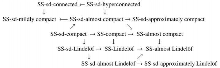
The aim of this study was to originate six types of generalized compactness and Lindelöfness in the frame of supra soft topological spaces (or SSTSs) based on the approaches of supra soft somewhere dense sets (or SS-sd-sets) and the SS-sd-closure operator, named SS-sd-almost compact (Lindelöf) spaces, SS-sd-approximately compact (Lindelöf) spaces and SS-sd-mildly compact (Lindelöf) spaces. The essential properties of each type of the aforementioned notions were studied. Specifically, we studied the invariance of these notions under specific types of soft mappings. Moreover, the relationships among these notions and between corresponding notions were discussed. Furthermore, the equivalence among them was proved under the SS-sd-partition condition. Finally, we provided a diagram to summarize these relationships with the support of concrete counterexamples.
Citation: Alaa M. Abd El-latif. Specific types of Lindelöfness and compactness based on novel supra soft operator[J]. AIMS Mathematics, 2025, 10(4): 8144-8164. doi: 10.3934/math.2025374
The aim of this study was to originate six types of generalized compactness and Lindelöfness in the frame of supra soft topological spaces (or SSTSs) based on the approaches of supra soft somewhere dense sets (or SS-sd-sets) and the SS-sd-closure operator, named SS-sd-almost compact (Lindelöf) spaces, SS-sd-approximately compact (Lindelöf) spaces and SS-sd-mildly compact (Lindelöf) spaces. The essential properties of each type of the aforementioned notions were studied. Specifically, we studied the invariance of these notions under specific types of soft mappings. Moreover, the relationships among these notions and between corresponding notions were discussed. Furthermore, the equivalence among them was proved under the SS-sd-partition condition. Finally, we provided a diagram to summarize these relationships with the support of concrete counterexamples.

| [1] |
D. A. Molodtsov, Soft set theory–first results, Comput. Math. Appl., 37 (1999), 19–31. https://doi.org/10.1016/S0898-1221(99)00056-5 doi: 10.1016/S0898-1221(99)00056-5

|
| [2] | P. K. Maji, R. Biswas, A. R. Roy, Soft set theory, Comput. Math. Appl., 45 (2003), 555–562. https://doi.org/10.1016/S0898-1221(03)00016-6 |
| [3] |
F. Karaaslan, Soft classes and soft rough classes with applications in decision making, Math. Probl. Eng., 2016 (2016), 1584528. https://doi.org/10.1155/2016/1584528 doi: 10.1155/2016/1584528
|
| [4] |
A. M. Abd El-latif, New Generalized fuzzy soft rough approximations applied to fuzzy topological spaces, J. Intell. Fuzzy Syst., 35 (2018), 2123–2136. https://doi.org/10.3233/JIFS-172076 doi: 10.3233/JIFS-172076
|
| [5] |
T. M. Al-shami, M. E. El-Shafei, Partial belong relation on soft separation axioms and decision making problem: two birds with one stone, Soft Comput., 24 (2020), 5377–5387. https://doi.org/10.1007/s00500-019-04295-7 doi: 10.1007/s00500-019-04295-7
|
| [6] |
N. Çagman, S. Enginoglu, Soft matrix theory and its decision making, Comput. Math. Appl., 59 (2010), 3308–3314. https://doi.org/10.1016/j.camwa.2010.03.015 doi: 10.1016/j.camwa.2010.03.015
|
| [7] |
S. Yuksel, T. Dizman, G. Yildizdan, U. Sert, Application of soft sets to diagnose the prostate cancer risk, J. Inequal. Appl., 2013 (2013), 229. https://doi.org/10.1186/1029-242X-2013-229 doi: 10.1186/1029-242X-2013-229
|
| [8] | A. Kharal, B. Ahmad, Mappings on soft classes, New Math. Nat. Comput., 7 (2011), 471–481. https://doi.org/10.1142/S1793005711002025 |
| [9] |
Z. A. Ameen, M. H. Alqahtani, Some classes of soft functions defined by soft open sets modulo soft sets of the first category, Mathematics, 11 (2023), 4368. https://doi.org/10.3390/math11204368 doi: 10.3390/math11204368
|
| [10] |
I. Zorlutuna, H. Çakir, On continuity of soft mappings, Appl. Math. Inform. Sci., 9 (2015), 403–409. https://doi.org/10.12785/amis/090147 doi: 10.12785/amis/090147
|
| [11] | Z. A. Ameen, A non-continuous soft mapping that preserves some structural soft sets, J. Intell. Fuzzy Syst., 42 (2022), 5839–5845. |
| [12] | M. Shabir, M. Naz, On soft topological spaces, Comput. Math. Appl., 61 (2011), 1786–1799. https://doi.org/10.1016/j.camwa.2011.02.006 |
| [13] | N. Çagman, S. Karataş, S. Enginoglu, Soft topology, Comput. Math. Appl., 62 (2011), 351–358. https://doi.org/10.1016/j.camwa.2011.05.016 |
| [14] | I. Arokiarani, A. A. Lancy, Generalized soft g$\beta$-closed sets and soft gs$\beta$-closed sets in soft topological spaces, International Journal of Mathematical Archive, 4 (2013), 17–23. |
| [15] | A. Kandil, O. A. E. Tantawy, S. A. El-Sheikh, A. M. A. El-latif, $\gamma$-Operation and decompositions of some forms of soft continuity in soft topological spaces, Annals of Fuzzy Mathematics and Informatics, 7 (2014), 181–196. |
| [16] | A. Kandil, O. A. E. Tantawy, S. A. El-Sheikh, A. M. Abd El-latif, Soft semi separation axioms and some types of soft functions, Annals of Fuzzy Mathematics and Informatics, 8 (2014), 305–318. |
| [17] | B. Chen, Soft semi-open sets and related properties in soft topological spaces, Appl. Math. Inform. Sci., 7 (2013), 36. |
| [18] |
T. M. Al-shami, A. Mhemdi, R. Abu-Gdairi, A novel framework for generalizations of soft open sets and its applications via soft topologies, Mathematics, 11 (2023), 840. https://doi.org/10.3390/math11040840 doi: 10.3390/math11040840
|
| [19] | S. A. El-sheikh, A. M. Abd El-latif, Characterization of b-open soft sets in soft topological spaces, Journal of New Theory, 2 (2015), 8–18. |
| [20] |
M. Akdag, A. Ozkan, Soft b-open sets and soft b-continuous functions, Math. Sci., 8 (2014), 124. https://doi.org/10.1007/s40096-014-0124-7 doi: 10.1007/s40096-014-0124-7
|
| [21] |
R. A. Abu-Gdairi, A. Azzam, I. Noaman, Nearly soft $\beta$-open sets via soft ditopological spaces, Eur. J. Pure Appl. Math., 15 (2022), 126–134. https://doi.org/10.29020/nybg.ejpam.v15i1.4249 doi: 10.29020/nybg.ejpam.v15i1.4249
|
| [22] |
S. Al Ghour, J. Al-Mufarrij, Between soft complete continuity and soft somewhat-continuity, Symmetry, 15 (2023), 2056. https://doi.org/10.3390/sym15112056 doi: 10.3390/sym15112056
|
| [23] |
T. M. Al-shami, Soft somewhere dense sets on soft topological spaces, Commun. Korean Math. S., 33 (2018), 1341–1356. https://doi.org/10.4134/CKMS.c170378 doi: 10.4134/CKMS.c170378
|
| [24] |
T. M. Al-shami, I. Alshammari, B. A. Asaad, Soft maps via soft somewhere dense sets, Filomat, 34 (2020), 3429–3440. https://doi.org/10.2298/FIL2010429A doi: 10.2298/FIL2010429A
|
| [25] |
A. M. Abd El-latif, A. A. Azzam, R. Abu-Gdairi, M. H. Alqahtani, G. M. Abd-Elhamed, Applications on soft somewhere dense sets, J. Interdiscip. Math., 27 (2024), 1679–1699. https://doi.org/10.47974/JIM-2007 doi: 10.47974/JIM-2007
|
| [26] |
Z. A. Ameen, R. Abu-Gdairi, T. M. Al-shami, B. A. Asaad, M. Arar, Further properties of soft somewhere dense continuous functions and soft Baire spaces, J. Math. Comput. Sci., 32 (2024), 54–63. https://doi.org/10.22436/jmcs.032.01.05 doi: 10.22436/jmcs.032.01.05
|
| [27] |
B. A. Asaad, T. M. Al-shami, Z. A. Ameen, On soft somewhere dense open functions and soft Baire spaces, Iraqi Journal of Science, 64 (2023), 373–384. https://doi.org/10.24996/ijs.2023.64.1.35 doi: 10.24996/ijs.2023.64.1.35
|
| [28] |
A. A. Azzam, Z. A. Ameen, T. M. Al-shami, M. E. El-Shafei, Generating soft topologies via soft set operators, Symmetry, 14 (2022), 914. https://doi.org/10.3390/sym14050914 doi: 10.3390/sym14050914
|
| [29] |
T. M. Al-shami, A. Mhemdi, R. Abu-Gdairi, M. E. El-Shafei, Compactness and connectedness via the class of soft somewhat open sets, AIMS Mathematics, 8 (2023), 815–840. https://doi.org/10.3934/math.2023040 doi: 10.3934/math.2023040
|
| [30] |
A. Kandil, O. A. E. Tantawy, S. A. El-Sheikh, A. M. Abd El-latif, Soft ideal theory, Soft local function and generated soft topological spaces, Appl. Math. Inform. Sci., 8 (2014), 1595–1603. https://doi.org/10.12785/amis/080413 doi: 10.12785/amis/080413
|
| [31] |
A. Kandil, O. A. E. Tantawy, S. A. El-Sheikh, A. M. Abd El-latif, Supra generalized closed soft sets with respect to an soft ideal in supra soft topological spaces, Appl. Math. Inform. Sci., 8 (2014), 1731–1740. http://doi.org/10.12785/amis/080430 doi: 10.12785/amis/080430
|
| [32] |
A. H. Hussain, S. A. Abbas, A. M. Salman, N. A. Hussein, Semi soft local function which generated a new topology in soft ideal spaces, J. Interdiscip. Math., 22 (2019), 1509–1517. https://doi.org/10.1080/09720502.2019.1706848 doi: 10.1080/09720502.2019.1706848
|
| [33] |
F. Gharib, A. M. Abd El-latif, Soft semi local functions in soft ideal topological spaces, Eur. J. Pure Appl. Math., 12 (2019), 857–869. https://doi.org/10.29020/nybg.ejpam.v12i3.3442 doi: 10.29020/nybg.ejpam.v12i3.3442
|
| [34] |
A. M. Abd El-latif, Generalized soft rough sets and generated soft ideal rough topological spaces, J. Intell. Fuzzy Syst., 34 (2018), 517–524. https://doi.org/10.3233/JIFS-17610 doi: 10.3233/JIFS-17610
|
| [35] | M. Akdag, F. Erol, Soft I-sets and soft I-continuity of functions, Gazi. U. J. Sci., 27 (2014), 923–932. |
| [36] | A. Kandil, O. A. E. Tantawy, S. A. El-sheikh, A. M. Abd El-latif, $\gamma$-Operation and decompositions of some forms of soft continuity of soft topological spaces via soft ideal, Annals of Fuzzy Mathematics and Informatics, 9 (2015), 385–402. |
| [37] |
A. A. Nasef, M. Parimala, R. Jeevitha, M. K. El-Sayed, Soft ideal theory and applications, Int. J. Nonlinear Anal., 13 (2022), 1335–1342. https://doi.org/10.22075/ijnaa.2022.6266 doi: 10.22075/ijnaa.2022.6266
|
| [38] |
Z. A. Ameen, M. H. Alqahtani, Congruence representations via soft ideals in soft topological spaces, Axioms, 12 (2023), 1015. https://doi.org/10.3390/axioms12111015 doi: 10.3390/axioms12111015
|
| [39] |
A. Kandil, O. A. E. Tantawy, S. A. El-sheikh, A. M. Abd El-latif, Soft regularity and normality based on semi open soft sets and soft ideals, Applied Mathematics and Information Sciences Letters, 3 (2015), 47–55. https://doi.org/10.12785/amisl/030202 doi: 10.12785/amisl/030202
|
| [40] | A. Kandil, O. A. E. Tantawy, S. A. El-sheikh, A. M. Abd El-latif, Soft semi (quasi) Hausdorff spaces via soft ideals, South Asian Journal of Mathematics, 4 (2014), 265–284. |
| [41] |
A. Aygünoǧlu, H. Aygün, Some notes on soft topological spaces, Neural Comput. Appl., 21 (2012), 113–119. https://doi.org/10.1007/s00521-011-0722-3 doi: 10.1007/s00521-011-0722-3
|
| [42] | T. Hida, A comprasion of two formulations of soft compactness, Annals of Fuzzy Mathematics and Informatics, 8 (2014), 511–525. |
| [43] |
A. Kandil, O. A. E. Tantawy, S. A. El-sheikh, A. M. Abd El-latif, Soft semi compactness via soft ideals, Appl. Math. Inform. Sci., 8 (2014), 2297–2306. https://doi.org/10.12785/amis/080524 doi: 10.12785/amis/080524
|
| [44] | A. Kandil, O. A. E. Tantawy, S. A. El-sheikh, A. M. Abd El-latif, Soft connectedness via soft ideals, Journal of New Results in Science, 4 (2014), 90–108. |
| [45] |
T. M. Al-Shami, A. Mhemdi, A. A. Rawshdeh, H. H. Al-Jarrah, Soft version of compact and Lindelof spaces using soft somewhere dense sets, AIMS Mathematics, 6 (2021), 8064–8077. https://doi.org/10.3934/math.2021468 doi: 10.3934/math.2021468
|
| [46] | S. A. El-sheikh, A. M. Abd El-latif, Decompositions of some types of supra soft sets and soft continuity, International Journal of Mathematics Trends and Technology, 9 (2014), 37–56. |
| [47] | A. M. Abd El-latif, S. Karataş, Supra $b$-open soft sets and supra $b$-soft continuity on soft topological spaces, Journal of Mathematics and Computer Applications Research, 5 (2015), 1–18. |
| [48] |
A. M. Abd El-latif, M. H. Alqahtani, New soft operators related to supra soft $\delta_i$-open sets and applications, AIMS Mathematics, 9 (2024), 3076–3096. https://doi.org/10.3934/math.2024150 doi: 10.3934/math.2024150
|
| [49] |
A. M. Abd El-latif, Novel types of supra soft operators via supra soft sd-sets and applications, AIMS Mathematics, 9 (2024), 6586–6602. https://doi.org/10.3934/math.2024321 doi: 10.3934/math.2024321
|
| [50] |
A. M. Abd El-latif, M. H. Alqahtani, Novel categories of supra soft continuous maps via new soft operators, AIMS Mathematics, 9 (2024), 7449-7470. https://doi.org/10.3934/math.2024361 doi: 10.3934/math.2024361
|
| [51] | A. M. Abd El-latif, R. Abu-Gdairi, A. A. Azzam, F. A. Gharib, K. A. Aldwoah, Supra soft somewhat open sets: characterizations and continuity, Eur. J. Pure Appl. Math., 18 (2025), 5863. |
| [52] |
A. M. Abd El-latif, On soft supra compactness in supra soft topological spaces, Tbilisi Math. J., 11 (2018), 169–178. https://doi.org/10.32513/tbilisi/1524276038 doi: 10.32513/tbilisi/1524276038
|
| [53] | A. M. Abd El-latif, R. A. Gdairi, A. A. Azzam, K. A. Aldwoah, M. Aldawood, S. M. Shaaban, Applications of the supra soft sd-closure operator to soft connectedness and compactness, Eur. J. Pure Appl. Math., 18 (2025), 5896. |
| [54] | I. Zorlutuna, M. Akdag, W. K. Min, S. Atmaca, Remarks on soft topological spaces, Annals of Fuzzy Mathematics and Informatics, 3 (2012), 171–185. |
| [55] |
A. M. Abd El-latif, A. A. Azzam, R. Abu-Gdairi, M. Aldawood, M. H. Alqahtani, New versions of maps and connected spaces via supra soft sd-operators, PLOS ONE, 19 (2024), e0304042. https://doi.org/10.1371/journal.pone.0304042 doi: 10.1371/journal.pone.0304042
|
| [56] |
T. M. Al-shami, On soft separation axioms and their applications on decision-making problem, Math. Probl. Eng., 2021 (2021), 8876978. https://doi.org/10.1155/2021/8876978 doi: 10.1155/2021/8876978
|
| [57] |
J. Sun, J. X. Zhang, L. Liu, Q. H. Shan, J. X. Zhang, Event-triggered consensus control of linear multi-agent systems under intermittent communication, J. Franklin I., 361 (2024), 106650. https://doi.org/10.1016/j.jfranklin.2024.106650 doi: 10.1016/j.jfranklin.2024.106650
|
| [58] |
J. Sun, J. X. Zhang, L. Liu, Y. M. Wu, Q. H. Shan, Output consensus control of multi-agent systems with switching networks and incomplete leader measurement, IEEE T. Autom. Sci. Eng., 21 (2024), 6643–6652. https://doi.org/10.1109/TASE.2023.3328897 doi: 10.1109/TASE.2023.3328897
|
| [59] |
T. M. Al-shami, A. Mhemdi, Approximation operators and accuracy measures of rough sets from an infra-topology view, Soft Comput., 27 (2023), 1317–1330. https://doi.org/10.1007/s00500-022-07627-2 doi: 10.1007/s00500-022-07627-2
|
| [60] |
A. M. Abd El-latif, Some properties of fuzzy supra soft topological spaces, Eur. J. Pure Appl. Math., 12 (2019), 999–1017. https://doi.org/10.29020/nybg.ejpam.v12i3.3440 doi: 10.29020/nybg.ejpam.v12i3.3440
|

Figures(2)

Alaa M. Abd El-latif. Specific types of Lindelöfness and compactness based on novel supra soft operator[J]. AIMS Mathematics, 2025, 10(4): 8144-8164. doi: 10.3934/math.2025374


 DownLoad: