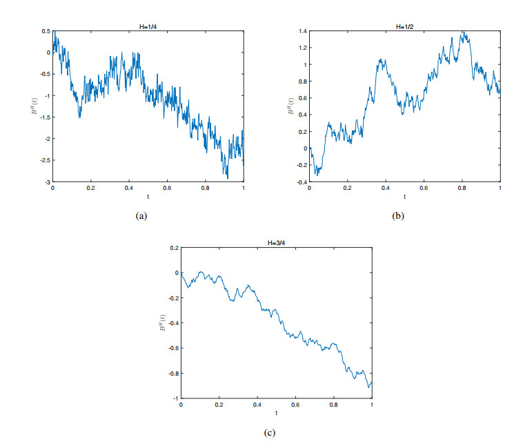
This paper presents a novel numerical method, named extended fractional neural stochastic differential equation (fNSDE)-Net, which combines the generative adversarial network (GAN) and fNSDE with a self-attention module. The method is designed to generate and forecast the stock price of Contemporary Amperex Technology Co., Ltd. (CATL) in China. The primary challenge of this study lies in the fact that the input consists of a single, irregular time-series dataset with long-range dependencies (i.e., Hurst index $ H > \frac{1}{2} $), and its inherent noise cannot be directly modeled using pure Brownian motion. The proposed method not only generates multiple sample paths based on the initial data in a probabilistic sense but also preserves the long-term memory characteristics of the generated samples. Moreover, the pricing of a Bermuda call option, induced by stock prices, is explored. Through a series of numerical error comparisons and estimator reliability tests, the proposed method outperforms both the pure fNSDE-GAN method and the NSDE-GAN method in terms of fitting and generalization performance, thereby demonstrating its effectiveness.
Citation: Xiao Qi, Tianyao Duan, Lihua Wang, Huan Guo. CATL's stock price forecasting and its derived option pricing: a novel extended fNSDE-net method[J]. AIMS Mathematics, 2025, 10(2): 2444-2465. doi: 10.3934/math.2025114
This paper presents a novel numerical method, named extended fractional neural stochastic differential equation (fNSDE)-Net, which combines the generative adversarial network (GAN) and fNSDE with a self-attention module. The method is designed to generate and forecast the stock price of Contemporary Amperex Technology Co., Ltd. (CATL) in China. The primary challenge of this study lies in the fact that the input consists of a single, irregular time-series dataset with long-range dependencies (i.e., Hurst index $ H > \frac{1}{2} $), and its inherent noise cannot be directly modeled using pure Brownian motion. The proposed method not only generates multiple sample paths based on the initial data in a probabilistic sense but also preserves the long-term memory characteristics of the generated samples. Moreover, the pricing of a Bermuda call option, induced by stock prices, is explored. Through a series of numerical error comparisons and estimator reliability tests, the proposed method outperforms both the pure fNSDE-GAN method and the NSDE-GAN method in terms of fitting and generalization performance, thereby demonstrating its effectiveness.

| [1] | H. Fan, Financial analysis in CATL based on Harvard analysis framework, 2022 2nd International Conference on Enterprise Management and Economic Development (ICEMED 2022), 2022,874–879. https://doi.org/10.2991/aebmr.k.220603.143 |
| [2] |
H. Liu, H. Liu, H. Wang, Research of power battery risk investment: taking CATL as an example, Financ. Eng. Risk Manag., 6 (2023), 5. https://doi.org/10.23977/ferm.2023.060501 doi: 10.23977/ferm.2023.060501

|
| [3] |
D. Lyu, Analyzing the risk-return trade-off relationship of Chinese new energy firms using the capital asset pricing model, High. Bus. Econ. Manag., 30 (2024), 429–435. https://doi.org/10.54097/fwj7mr52 doi: 10.23977/ferm.2023.060501
|
| [4] | K. Hayashi, K. Nakagawa, Fractional SDE-net: generation of time series data with long-term memory, 2022 IEEE 9th International Conference on Data Science and Advanced Analytics (DSAA), 2022. https://doi.org/10.1109/DSAA54385.2022.10032351 |
| [5] | P. Kidger, J. Foster, X. Li, T. J. Lyons, Neural SDEs as infinite-dimensional GANs, International Conference on Machine Learning, 2021, 5453–5463. Available form: https://proceedings.mlr.press/v139/kidger21b.html. |
| [6] |
F. A. Longstaff, E. S. Schwartz, Valuing American options by simulation: a simple least-squares approach, Rev. Financ. Stud., 14 (2001), 113–147. https://doi.org/10.1093/rfs/14.1.113 doi: 10.1093/rfs/14.1.113
|
| [7] |
P. A. Sadorsky, A random forests approach to predicting clean energy stock prices, J. Risk. Financ. Manag., 14 (2021), 48. https://doi.org/10.3390/jrfm14020048 doi: 10.3390/jrfm14020048
|
| [8] |
P. A. Sadorsky, Forecasting solar stock prices using tree-based machine learning classification: How important are silver prices? North Amer. J. Econ. Finance, 61 (2022), 101705. https://doi.org/10.1016/j.najef.2022.101705 doi: 10.1016/j.najef.2022.101705
|
| [9] |
M. Wang, Z. Xiao, H. Peng, X. Wang, J. Wang, Stock price prediction for new energy vehicle enterprises: an integrated method based on time series and cloud models, Expert. Syst. Appl., 208 (2022), 118125. https://doi.org/10.1016/j.eswa.2022.118125 doi: 10.1016/j.eswa.2022.118125
|
| [10] |
L. Gu, C. Feng, Research on stock price prediction based on Markov-LSTM neural network-take the new energy industry as an example, Acad. J. Bus. Manag., 4 (2022), 42–47. https://doi.org/10.25236/AJBM.2022.040408 doi: 10.25236/AJBM.2022.040408
|
| [11] |
A. Meng, P. Wang, G. Zhai, C. Zeng, S. Chen, X. Yang, et al., Electricity price forecasting with high penetration of renewable energy using attention-based LSTM network trained by crisscross optimization, Energy, 254 (2022), 124212. https://doi.org/10.1016/j.energy.2022.124212 doi: 10.1016/j.energy.2022.124212
|
| [12] |
Q. Shen, Y. Zhang, J. Xiao, X. Dong, Z. Lin, Research of daily stock closing price prediction for new energy companies in China, Data. Sci. Finance Econ., 3 (2023), 14–29. https://doi.org/10.3934/DSFE.2023002 doi: 10.3934/DSFE.2023002
|
| [13] |
Q. Zhu, X. Zhou, S. Liu, High return and low risk: shaping composite financial investment decision in the new energy stock market, Energy Econ., 122, (2023), 106683. https://doi.org/10.1016/j.eneco.2023.106683 doi: 10.1016/j.eneco.2023.106683
|
| [14] |
G. F. Fan, R. T. Zhang, C. C. Cao, L. L. Peng, Y. H. Yeh, W. C. Hong, The volatility mechanism and intelligent fusion forecast of new energy stock prices, Financ. Innov., 10 (2024), 84. https://doi.org/10.1186/s40854-024-00621-7 doi: 10.1186/s40854-024-00621-7
|
| [15] | M. M. Alshater, I. Kampouris, H. Marashdeh, O. F. Atayah, H. Banna, Early warning system to predict energy prices: the role of artificial intelligence and machine learning, Ann. Oper. Res., 2022. https://doi.org/10.1007/s10479-022-04908-9 |
| [16] |
H. Gao, G. Kou, H. Liang, H. Zhang, X. Chao, C. Li, Y. Dong, Machine learning in business and finance: a literature review and research opportunities, Financ. Innov., 10 (2024), 86. https://doi.org/10.1186/s40854-024-00629-z doi: 10.1186/s40854-024-00629-z
|
| [17] |
I. Ghosh, R. K. Jana, Clean energy stock price forecasting and response to macroeconomic variables: a novel framework using Facebook's prophet, neuralprophet and explainable AI, Technol. Forecast. Soc. Change, 200 (2024), 123148. https://doi.org/10.1016/j.techfore.2023.123148 doi: 10.1016/j.techfore.2023.123148
|
| [18] | L. Jiang, G. Hu, A review on short-term electricity price forecasting techniques for energy markets, 2018 15th International Conference on Control, Automation, Robotics and Vision (ICARCV), 2018,937–944. https://doi.org/10.1109/ICARCV.2018.8581312 |
| [19] |
Y. Lin, Q. Lu, B. Tan, Y. Yu, Forecasting energy prices using a novel hybrid model with variational mode decomposition, Energy, 246 (2023), 123366. https://doi.org/10.1016/j.energy.2022.123366 doi: 10.1016/j.energy.2022.123366
|
| [20] |
M. M. Mostafa, A. A. El-Masry, Oil price forecasting using gene expression programming and artificial neural networks, Econ. Model., 54 (2016), 40–53. https://doi.org/10.1016/j.econmod.2015.12.014 doi: 10.1016/j.econmod.2015.12.014
|
| [21] |
R. Pino, J. Parreno, A. Gomez, P. Priore, Forecasting next-day price of electricity in the Spanish energy market using artificial neural networks, Eng. Appl. Artif. Intell., 21 (2008), 53–62. https://doi.org/10.1016/j.engappai.2007.02.001 doi: 10.1016/j.engappai.2007.02.001
|
| [22] | G. J. Lord, C. E. Powell, T. Shardlow, An introduction to computational stochastic PDEs, Cambridge University Press, 2014. https://doi.org/10.1017/CBO9781139017329 |
| [23] | F. Biagini, Y. Hu, B. Øksendal, T. Zhang, Stochastic calculus for fractional Brownian motion and applications, Springer Science & Business Media Publishers, 2008. https://doi.org/10.1007/978-1-84628-797-8 |
| [24] | X. An, X. Yi, B. Zhou, Q. Zhang, Research on stock market investment model based on time series forecasting and dynamic programming, Proceedings of the 3rd International Conference on Internet Finance and Digital Economy (ICIFDE 2023), 2023,412–420. https://doi.org/10.2991/978-94-6463-270-5_46 |
| [25] |
T. Wang, J. Guo, Y. Shan, Y. Zhang, B. Peng, Z. Wu, A knowledge graph-GCN-community detection integrated model for large-scale stock price prediction, Appl. Soft. Comput., 145 (2023), 110595. https://doi.org/10.1016/j.asoc.2023.110595 doi: 10.1016/j.asoc.2023.110595
|
| [26] | B. Mandelbrot, Statistical methodology for nonperiodic cycles: from the covariance to R/S analysis, Nber, 1972,259–290. |
| [27] |
M. J. Wainwright, M. I. Jordan, Graphical models, exponential families, and variational inference, Found. Trends Mach. Learn., 1 (2008), 1–305. https://doi.org/10.1561/2200000001 doi: 10.1561/2200000001
|
| [28] | H. Zhang, I. Goodfellow, D. Metaxas, A. Odena, Self-attention generative adversarial networks, Proceedings of the 36th International Conference on Machine Learning, 2019. |
| [29] | P. Kidger, J. Morrill, J. Foster, T. Lyons, Neural controlled differential equations for irregular time series, Adv. Neural Inf. Process. Syst., 33 (2020), 6696–6707. |
| [30] | M. Arjovsky, S. Chintala, L. Bottou, Wasserstein generative adversarial networks, ICML'17: Proceedings of the 34th International Conference on Machine Learning, 70 (2017), 214–223. |
| [31] | I. Goodfellow, J. Pouget-Abadie, M. Mirza, B. Xu, D. Warde-Farley, S. Ozair, et al., Generative adversarial nets, Adv. Neural Inf. Process. Syst., 2 (2021), 2672–2680. |
| [32] | X. Li, T. K. L. Wong, R. T. Chen, D. K. Duvenaud, Scalable gradients and variational inference for stochastic differential equations, Proceedings of the Twenty Third International Conference on Artificial Intelligence and Statistics, 2020. |
| [33] |
A. Q. Md, S. Kapoor, A. V. C. Junni, A. K. Sivaraman, K. F. Tee, H. Sabireen, et al., Novel optimization approach for stock price forecasting using multi-layered sequential LSTM, Appl. Soft Comput., 134 (2023), 109830. https://doi.org/10.1016/j.asoc.2022.109830 doi: 10.1016/j.asoc.2022.109830
|
| [34] |
U. S. M. de Lima, C. P. Samanez, Complex derivatives valuation: applying the least-squares Monte Carlo simulation method with several polynomial basis, Financ. Innov., 2 (2018), 1. https://doi.org/10.1186/s40854-015-0019-0 doi: 10.1186/s40854-015-0019-0
|


Figures(4) / Tables(16)

Xiao Qi, Tianyao Duan, Lihua Wang, Huan Guo. CATL's stock price forecasting and its derived option pricing: a novel extended fNSDE-net method[J]. AIMS Mathematics, 2025, 10(2): 2444-2465. doi: 10.3934/math.2025114


 DownLoad: