Chen considered the existence of a Hamiltonian cycle containing a matching and avoiding some edges in an $ n $-cube $ Q_n $. In this paper, we considered the existence of a Hamiltonian path and obtained the following result. For $ n\geq4 $, let $ M $ be a matching of $ Q_n $, and let $ F $ be a set of edges in $ Q_n-M $ with $ |M\cup F|\leq2n-6 $. Let $ x $ and $ y $ be two vertices of $ Q_n $ with different parities satisfying $ xy\notin M $. If all vertices in $ Q_n-F $ have a degree of at least $ 2 $, then there exists a Hamiltonian path joining $ x $ and $ y $ passing through $ M $ in $ Q_n-F $, with the exception of two cases: (1) there exist two neighbors $ v $ and $ t $ of $ x $ (or $ y $) satisfying $ d_{Q_n-F}(v) = 2 $ and $ xt\in M $ (or $ yt\in M $); (2) there exists a path $ xvuy $ of length 3 satisfying $ d_{Q_n-F}(v) = 2 $ and $ uy\in M $ or $ d_{Q_n-F}(u) = 2 $ and $ xv\in M $.
Citation: Shenyang Zhao, Fan Wang. Hamiltonian paths passing through matchings in hypercubes with faulty edges[J]. AIMS Mathematics, 2024, 9(12): 33692-33711. doi: 10.3934/math.20241608
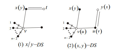
Chen considered the existence of a Hamiltonian cycle containing a matching and avoiding some edges in an $ n $-cube $ Q_n $. In this paper, we considered the existence of a Hamiltonian path and obtained the following result. For $ n\geq4 $, let $ M $ be a matching of $ Q_n $, and let $ F $ be a set of edges in $ Q_n-M $ with $ |M\cup F|\leq2n-6 $. Let $ x $ and $ y $ be two vertices of $ Q_n $ with different parities satisfying $ xy\notin M $. If all vertices in $ Q_n-F $ have a degree of at least $ 2 $, then there exists a Hamiltonian path joining $ x $ and $ y $ passing through $ M $ in $ Q_n-F $, with the exception of two cases: (1) there exist two neighbors $ v $ and $ t $ of $ x $ (or $ y $) satisfying $ d_{Q_n-F}(v) = 2 $ and $ xt\in M $ (or $ yt\in M $); (2) there exists a path $ xvuy $ of length 3 satisfying $ d_{Q_n-F}(v) = 2 $ and $ uy\in M $ or $ d_{Q_n-F}(u) = 2 $ and $ xv\in M $.

| [1] | J. Bondy, U. Murty, Graph Theory with Applications, London: Macmillan Press, 1976. |
| [2] |
R. Caha, V. Koubek, Hamiltonian cycles and paths with a prescribed set of edges in hypercubes and dense sets, J. Graph Theory, 51 (2006), 137–169. https://doi.org/10.1002/jgt.20128 doi: 10.1002/jgt.20128

|
| [3] |
R. Caha, V. Koubek, Spanning multi-paths in hypercubes, Discrete Math., 307 (2007), 2053–2066. https://doi.org/10.1016/j.disc.2005.12.050 doi: 10.1016/j.disc.2005.12.050
|
| [4] |
X. Chen, Paired many-to-many disjoint path covers of hypercubes with faulty edges, Inform. Process. Lett., 112 (2012), 61–66. https://doi.org/10.1016/j.ipl.2011.10.010 doi: 10.1016/j.ipl.2011.10.010
|
| [5] |
X. Chen, Matchings extend to Hamiltonian cycles in hypercubes with faulty edges, Front. Math. China, 14 (2019), 1117–1132. https://doi.org/10.1007/s11464-019-0810-8 doi: 10.1007/s11464-019-0810-8
|
| [6] |
D. Dimitrov, T. Dvořák, P. Gregor, R. Škrekovski, Gray codes avoiding matchings, Discrete Math. Theor. Comput. Sci., 11 (2009), 123–148. https://doi.org/10.46298/dmtcs.457 doi: 10.46298/dmtcs.457
|
| [7] |
T. Dvořák, Hamiltonian cycles with prescribed edges in hypercubes, SIAM J. Discrete Math., 19 (2005), 135–144. https://doi.org/10.1137/S0895480103432805 doi: 10.1137/S0895480103432805
|
| [8] |
T. Dvořák, P. Gregor, Hamiltonian paths with prescribed edges in hypercubes, Discrete Math., 307 (2007), 1982–1998. https://doi.org/10.1016/j.disc.2005.12.045 doi: 10.1016/j.disc.2005.12.045
|
| [9] |
J. Fink, Perfect matchings extend to Hamilton cycles in hypercubes, J. Combin. Theory Ser. B, 97 (2007), 1074–1076. https://doi.org/10.1016/j.jctb.2007.02.007 doi: 10.1016/j.jctb.2007.02.007
|
| [10] |
J. Fink, Connectivity of matching graph of hypercube, SIAM J. Discrete Math., 23 (2009), 1100–1109. https://doi.org/10.1137/070697288 doi: 10.1137/070697288
|
| [11] |
P. Gregor, Perfect matchings extending on subcubes to Hamiltonian cycles of hypercubes, Discrete Math., 309 (2009), 1711–1713. https://doi.org/10.1016/j.disc.2008.02.013 doi: 10.1016/j.disc.2008.02.013
|
| [12] | L. Gros, Théorie du Baguenodier, Lyon: Aimé Vingtrinier, 1872. |
| [13] | I. Havel, On Hamiltonian circuits and spanning trees of hypercube, Čas. Pěst. Mat., 109 (1984), 135–152. http://dml.cz/dmlcz/108506 |
| [14] | G. Kreweras, Matchings and hamiltonian cycles on hypercubes, Bull. Inst. Combin. Appl., 16 (1996), 87–91. |
| [15] |
M. Lewinter, W. Widulski, Hyper-Hamilton laceable and caterpillar-spannable product graphs, Comput. Math. Appl., 34 (1997), 99–104. https://doi.org/10.1016/S0898-1221(97)00223-X doi: 10.1016/S0898-1221(97)00223-X
|
| [16] |
J. J. Liu, Y. L. Wang, Hamiltonian cycles in hypercubes with faulty edges, Inform. Sci., 256 (2014), 225–233. https://doi.org/10.1016/j.ins.2013.09.012 doi: 10.1016/j.ins.2013.09.012
|
| [17] |
C. Tsai, Linear array and ring embeddings in conditional faulty hypercubes, Theor. Comput. Sci., 314 (2004), 431–443. https://doi.org/10.1016/j.tcs.2004.01.035 doi: 10.1016/j.tcs.2004.01.035
|
| [18] |
C. Tsai, Y. Lai, Conditional edge-fault-tolerant edge-bipancyclicity of hypercubes, Inform. Sci., 177 (2007), 5590–5597. https://doi.org/10.1016/j.ins.2007.06.013 doi: 10.1016/j.ins.2007.06.013
|
| [19] |
W. Wang, X. Chen, A fault-free Hamiltonian cycle passing through prescribed edges in a hypercube with faulty edges, Inform. Process. Lett., 107 (2008), 205–210. https://doi.org/10.1016/j.ipl.2008.02.016 doi: 10.1016/j.ipl.2008.02.016
|
| [20] |
F. Wang, H. P. Zhang, Small matchings extend to Hamiltonian cycles in hypercubes, Graphs Combin., 32 (2016), 363–376. https://doi.org/10.1007/s00373-015-1533-6 doi: 10.1007/s00373-015-1533-6
|
| [21] |
F. Wang, H. P. Zhang, Hamiltonian laceability in hypercubes with faulty edges, Discrete Appl. Math., 236 (2018), 438–445. https://doi.org/10.1016/j.dam.2017.10.005 doi: 10.1016/j.dam.2017.10.005
|
| [22] |
J. M. Xu, Z. Z. Du, M. Xu, Edge-fault-tolerant edge-bipancyclicity of hypercubes, Inform. Process. Lett., 96 (2005), 146–150. https://doi.org/10.1016/j.ipl.2005.06.006 doi: 10.1016/j.ipl.2005.06.006
|
| [23] |
Y. Yang, N. Song, Z. Zhao, Hamiltonian Laceability of Hypercubes with Prescribed Linear Forest and/or Faulty Edges, J. Combinat. Math. Combinat. Comput., 120 (2024), 393–398. https://doi.org/10.61091/jcmcc120-36 doi: 10.61091/jcmcc120-36
|


Figures(5)

Shenyang Zhao, Fan Wang. Hamiltonian paths passing through matchings in hypercubes with faulty edges[J]. AIMS Mathematics, 2024, 9(12): 33692-33711. doi: 10.3934/math.20241608


 DownLoad: