Visual Methodologies and Geography's education in the pandemic time: notes on geopolitics of migration in the "Mediterranean Complex"

Gabriella Palermo; Gabriella Palermo

doi:10.3934/geosci.2022015

AIMS Geosciences

2022, Volume 8, Issue 2: 254-265. doi: 10.3934/geosci.2022015

Previous Article Next Article

Research article Special Issues

Visual Methodologies and Geography's education in the pandemic time: notes on geopolitics of migration in the "Mediterranean Complex"

Gabriella Palermo ^,

Department of Culture e Società, Università degli studi di Palermo, Palermo, Italy

Received: 03 February 2022 Revised: 21 March 2022 Accepted: 27 March 2022 Published: 06 April 2022

The relationship between Geography and the Visual has always been strong intertwined. As it is true that Geography has always operates through images (in the form of pictures, creative representations and above all cartographies), in the last two years, with the distance learning due to the spread of the Covid-19 pandemic, this phenomenon has not only increased, but it also became necessary. "The classroom as the most radical space", in the words of bell hooks, had to turn into a virtual space, where images have a fundamental role in the teaching/learning process. This paper wants to analyse the relationship between Geography and the Visual by analysing three images we used in the lessons of the course Geopolitics of Migration at the University of Palermo during the academic year 2020–2021, that speak about the "Mediterranean Complex". With this expression, inspired by Mirzoeff's work, I will briefly focus on the clash between dominant visuality and the counter-visualities emerging from the Mediterranean Sea, a particular sea-space where on the one hand, violent geopolitics daily act against migrants' crossing; on the other hand, new imaginative geographies emerge against coloniality devices of power and knowledge. A further reflection will be dedicated to the use of these images as a didactic tool. Why do we use these images? What do they tell us? Which one is the relationship between our increasingly digital classrooms and these images? If it is true that the pandemic phenomenon is acting as a laboratory of experimentation and acceleration, how is the visual nature of geography changing and participating to the construction of our knowledge? This contribution is a first attempt to reflect about those questions through the visuality and the counter-visualities of the "Mediterranean complex".
- visual geography,
- education,
- Covid-19,
- counter-visualities,
- Mediterranean complex
Citation: Gabriella Palermo. Visual Methodologies and Geography's education in the pandemic time: notes on geopolitics of migration in the 'Mediterranean Complex'[J]. AIMS Geosciences, 2022, 8(2): 254-265. doi: 10.3934/geosci.2022015

Related Papers:

Abstract

The relationship between Geography and the Visual has always been strong intertwined. As it is true that Geography has always operates through images (in the form of pictures, creative representations and above all cartographies), in the last two years, with the distance learning due to the spread of the Covid-19 pandemic, this phenomenon has not only increased, but it also became necessary. "The classroom as the most radical space", in the words of bell hooks, had to turn into a virtual space, where images have a fundamental role in the teaching/learning process. This paper wants to analyse the relationship between Geography and the Visual by analysing three images we used in the lessons of the course Geopolitics of Migration at the University of Palermo during the academic year 2020–2021, that speak about the "Mediterranean Complex". With this expression, inspired by Mirzoeff's work, I will briefly focus on the clash between dominant visuality and the counter-visualities emerging from the Mediterranean Sea, a particular sea-space where on the one hand, violent geopolitics daily act against migrants' crossing; on the other hand, new imaginative geographies emerge against coloniality devices of power and knowledge. A further reflection will be dedicated to the use of these images as a didactic tool. Why do we use these images? What do they tell us? Which one is the relationship between our increasingly digital classrooms and these images? If it is true that the pandemic phenomenon is acting as a laboratory of experimentation and acceleration, how is the visual nature of geography changing and participating to the construction of our knowledge? This contribution is a first attempt to reflect about those questions through the visuality and the counter-visualities of the "Mediterranean complex".

References

[1]	Bignante E (2011) Geografia e ricerca visuale: strumenti e metodi, Roma-Bari: Laterza.
[2]	Heidegger M (2003) Die Zeit des Weltbildes, Frankfurt am Main: Klostermann.
[3]	Sloterdijk P (2005) Im Weltinnenraum des Kapitals, Frankfurt am Main: Suhrkamp Verlag.
[4]	De Spuches G (2015) Le esposizioni universali: spazialità e politiche di rappresentazione, Ric Storiche 45: 105–114.
[5]	Spivak GC (1988) Can the Subaltern Speak? Marxism and the Interpretation of Culture, Champaign: University of Illinois Press, 271–313.
[6]	Mirzoeff N (2011) The Right to Look. A Counterhistory of Visuality, Durham: Duke University Press.
[7]	Vallorani N (2017) Nessun Kurtz. Cuore di tenebra e le parole dell'Occidente, Milano: Mimesis.
[8]	Sharpe C (2016) In the Wake: on Blackness and Being, Durham: Duke University Press.
[9]	Rose G (2016) Visual Methodologies. An Introduction to Researching with Visual Materials, 4^th Edition, New York: Sage Publishing.
[10]	Cosgrove D, (2008) Geography and Vision. Seeing, Imagining and Representing the World, London-New York: I.B. Tauris and Co.
[11]	Haraway DJ (1991) Simians, Cyborgs, and Women, New York: Routledge.
[12]	Hughes R (2007) Through the Looking Blast: Geopolitics and Visual Culture. Geogr Compass 1: 976–994. https://doi.org/10.1111/j.1749-8198.2007.00052.x doi: 10.1111/j.1749-8198.2007.00052.x
[13]	Crang M (2009) Visual Methods and Methodologies. In: DeLyser D (eds.) The SAGE Handbook of Qualitative Geography, New York: Sage Publishing, 208–225.
[14]	Rose G (2003) On the Need to Ask How, Exactly, is Geography "Visual"? Antipode 35: 212–221. https://doi.org/10.1111/1467-8330.00317. doi: 10.1111/1467-8330.00317
[15]	De Spuches G, Sabatini F, Palermo G, et al. (2020) Risk narrations and perceptions in the Covid-19 time. A discourse analysis through the Italian press. AIMS Geosci 6: 504–514. https://doi.org/10.3934/geosci.2020028 doi: 10.3934/geosci.2020028
[16]	Palmentieri S (2022) E-Learning in Geography: new perspectives in post-pandemic. AIMS Geosci 8: 52–67. https://doi.org/10.3934/geosci.2022004 doi: 10.3934/geosci.2022004
[17]	Hooks B (1994) Teaching to transgress. Education as the Practice of Freedom, New York: Routledge.
[18]	Haraway DJ (2016) Staying with the Trouble. Making Kin in the Chthulucene, Durham: Duke University Press.
[19]	Rinella A (2019) Cinema, narrazione delle guerre e discorso geopolitico: riflessioni metodologiche e proposte didattiche In: Salvatori F (ed.) L'apporto della Geografia tra rivoluzioni e riforme. Atti del XXXII Congresso Geografico Italiano, Roma: A.Ge.I., 2123–2129. Available from: https://www.ageiweb.it/wp-content/uploads/2019/02/S29_p.pdf.
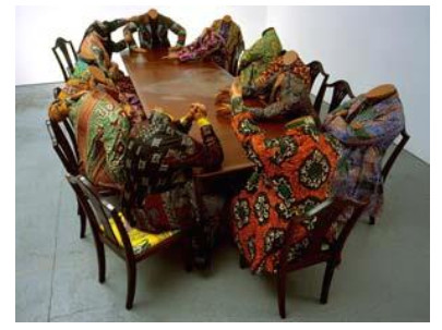
[20]	Smithsonian National Museum of African Art, Exhibition by Yinka Shonibare. Available from: https://africa.si.edu/exhibits/shonibare/scramble.html
[21]	Harley JB (2011) Deconstructing the Map, The Map Reader. Theories of Mapping Practice and Cartographic Representation, Hoboken: Wiley-Blackwell. https://doi.org/10.1002/9780470979587
[22]	Ó Tuathail G, Dalby S, Routledge P (1997) The Geopolitics Reader, New York: Routledge.
[23]	Mbembe A (2003) Necropolitics. Public Culture 15: 11–40. https://doi.org/10.1215/08992363-15-1-11 doi: 10.1215/08992363-15-1-11
[24]	de Spuches G, Palermo G (2020) Between Wakes and Waves: An Anti-Geopolitical View of a Postcolonial Mediterranean Space, In Favarò V, Marcenò S, Rethinking Borders. Decolonizing Knowledge and Categories, Palermo: Palermo University Press, 33–60.

Reader Comments

Your name:*

Email:*
© 2022 the Author(s), licensee AIMS Press. This is an open access article distributed under the terms of the Creative Commons Attribution License (http://creativecommons.org/licenses/by/4.0)