It is important to classify electroencephalography (EEG) signals automatically for the diagnosis and treatment of epilepsy. Currently, the dominant single-modal feature extraction methods cannot cover the information of different modalities, resulting in poor classification performance of existing methods, especially the multi-classification problem. We proposed a multi-modal feature fusion (MMFF) method for epileptic EEG signals. First, the time domain features were extracted by kernel principal component analysis, the frequency domain features were extracted by short-time Fourier extracted transform, and the nonlinear dynamic features were extracted by calculating sample entropy. On this basis, the features of these three modalities were interactively learned through the multi-head self-attention mechanism, and the attention weights were trained simultaneously. The fused features were obtained by combining the value vectors of feature representations, while the time, frequency, and nonlinear dynamics information were retained to screen out more representative epileptic features and improve the accuracy of feature extraction. Finally, the feature fusion method was applied to epileptic EEG signal classifications. The experimental results demonstrated that the proposed method achieves a classification accuracy of 92.76 ± 1.64% across the five-category classification task for epileptic EEG signals. The multi-head self-attention mechanism promotes the fusion of multi-modal features and offers an efficient and novel approach for diagnosing and treating epilepsy.
Citation: Ning Huang, Zhengtao Xi, Yingying Jiao, Yudong Zhang, Zhuqing Jiao, Xiaona Li. Multi-modal feature fusion with multi-head self-attention for epileptic EEG signals[J]. Mathematical Biosciences and Engineering, 2024, 21(8): 6918-6935. doi: 10.3934/mbe.2024304
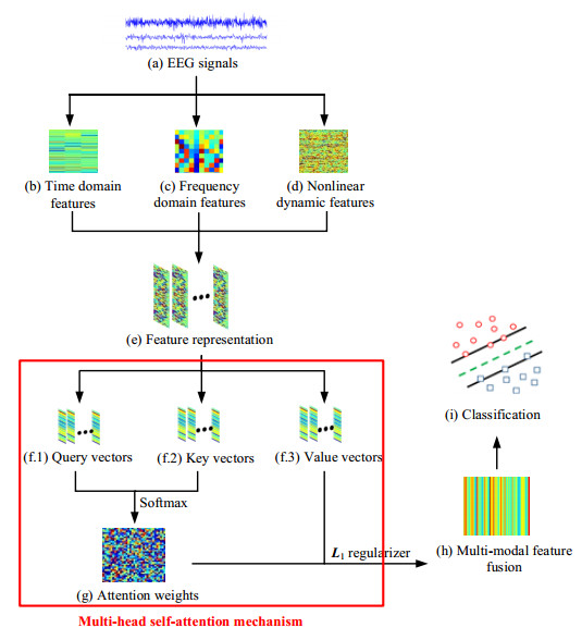
It is important to classify electroencephalography (EEG) signals automatically for the diagnosis and treatment of epilepsy. Currently, the dominant single-modal feature extraction methods cannot cover the information of different modalities, resulting in poor classification performance of existing methods, especially the multi-classification problem. We proposed a multi-modal feature fusion (MMFF) method for epileptic EEG signals. First, the time domain features were extracted by kernel principal component analysis, the frequency domain features were extracted by short-time Fourier extracted transform, and the nonlinear dynamic features were extracted by calculating sample entropy. On this basis, the features of these three modalities were interactively learned through the multi-head self-attention mechanism, and the attention weights were trained simultaneously. The fused features were obtained by combining the value vectors of feature representations, while the time, frequency, and nonlinear dynamics information were retained to screen out more representative epileptic features and improve the accuracy of feature extraction. Finally, the feature fusion method was applied to epileptic EEG signal classifications. The experimental results demonstrated that the proposed method achieves a classification accuracy of 92.76 ± 1.64% across the five-category classification task for epileptic EEG signals. The multi-head self-attention mechanism promotes the fusion of multi-modal features and offers an efficient and novel approach for diagnosing and treating epilepsy.

| [1] |
L. Chen, W. Q. Yang, F. Yang, Y. Y. Yu, T. W. Xu, D. Wang, et al., The crosstalk between epilepsy and dementia: A systematic review and meta-analysis, Epilepsy Behav., 152 (2024), 109640. https://doi.org/10.1016/j.yebeh.2024.109640 doi: 10.1016/j.yebeh.2024.109640

|
| [2] |
D. R. Nordli, K. Fives, F. Galan, Portable headband electroencephalogram in the detection of absence epilepsy, Clin. EEG Neurosci., 55 (2024), 581-585. https://doi.org/10.1177/15500594241229153 doi: 10.1177/15500594241229153
|
| [3] |
R. Qian, Z. G. Wu, The application of video electroencephalogram in the classification and diagnosis of post-stroke epilepsy, Clin. Neurosci. Res., 1 (2023), 37-41. https://doi.org/10.26689/cnr.v1i3.5849 doi: 10.26689/cnr.v1i3.5849
|
| [4] |
J. Li, X. L. Kong, L. L. Sun, X. Chen, G. X. Ouyang, X. L. Li, et al., Identification of autism spectrum disorder based on electroencephalography: A systematic review, Comput. Biol. Med., 170 (2024), 108075. https://doi.org/10.1016/j.compbiomed.2024.108075 doi: 10.1016/j.compbiomed.2024.108075
|
| [5] |
B. Boashash, S. Ouelha, Automatic signal abnormality detection using time-frequency features and machine learning: A newborn EEG seizure case study, Knowl. Based Syst., 106 (2016), 38-50. https://doi.org/10.1016/j.knosys.2016.05.027 doi: 10.1016/j.knosys.2016.05.027
|
| [6] |
S. A. Irimiciuc, A. Zala, D. Dimitriu, L. M. Himiniuc, M. Agop, B. F. Toma, et al., Novel approach for EEG signal analysis in a multifractal paradigm of motions. Epileptic and eclamptic seizures as scale transitions, Symmetry, 13 (2021), 1024. https://doi.org/10.3390/sym13061024 doi: 10.3390/sym13061024
|
| [7] |
M. Sabeti, S. Katebi, R. Boostani, Entropy and complexity measures for EEG signal classification of schizophrenic and control participants, Artif. Intell. Med., 47 (2009), 263-274. https://doi.org/10.1016/j.artmed.2009.03.003 doi: 10.1016/j.artmed.2009.03.003
|
| [8] |
M. Khayretdinova, I. Zakharov, P. Pshonkovskaya, T. Adamovich, A. Kiryasov, A. Zhdanov, et al., Prediction of brain sex from EEG: using large-scale heterogeneous dataset for developing a highly accurate and interpretable ML model, NeuroImage, 285 (2024), 120495. https://doi.org/10.1016/j.neuroimage.2023.120495 doi: 10.1016/j.neuroimage.2023.120495
|
| [9] | K. Prantzalos, D. Upadhyaya, N. Shafiabadi, G. Fernandez-BacaVaca, N. Gurski, K. Yoshimoto, et al., MaTiLDA: An integrated machine learning and topological data analysis platform for brain network dynamics, Pac. Symp. Biocomput. 2024, (2023), 65-80. https://doi.org/10.1142/9789811286421_0006 |
| [10] | S. V. J, L. J. J, P. P. R, Depression detection in working environment using 2D CSM and CNN with EEG signals, in 2022 9th International Conference on Computing for Sustainable Global Development (INDIACom), (2022), 722-726. https://doi.org/10.23919/INDIACom54597.2022.9763173 |
| [11] |
A. Seal, R. Bajpai, J. Agnihotri, A. Yazidi, E. Herrera-Viedma, O. Krejcar, DeprNet: A deep convolution neural network framework for detecting depression using EEG, IEEE Trans. Instrum. Meas., 70 (2021), 1-13. https://doi.org/10.1109/TIM.2021.3053999 doi: 10.1109/TIM.2021.3053999
|
| [12] |
N. Zrira, A. Kamal-Idrissi, R. Farssi, H. A. Khan, Time series prediction of sea surface temperature based on BiLSTM model with attention mechanism, J. Sea Res., 198 (2024), 102472. https://doi.org/10.1016/j.seares.2024.102472 doi: 10.1016/j.seares.2024.102472
|
| [13] |
J. Yang, M. Awais, A. Hossain, P. L. Yee, M. Haowei, I. M. Mehedi, et al., Thoughts of brain EEG signal-to-text conversion using weighted feature fusion-based multiscale dilated adaptive densenet with attention mechanism, Biomed. Signal Process., 86 (2023), 105120. https://doi.org/10.1016/j.bspc.2023.105120 doi: 10.1016/j.bspc.2023.105120
|
| [14] |
X. Zheng, W. Z. Chen, An attention-based bi-LSTM method for visual object classification via EEG, Biomed. Signal Process., 63 (2021), 102174. https://doi.org/10.1016/j.bspc.2020.102174 doi: 10.1016/j.bspc.2020.102174
|
| [15] |
B. X. Zhang, W. K. Li, Real-time emotion classification model for few-channel EEG signals, J. Chin. Comput. Syst., 45 (2024), 271-277. https://doi.org/10.20009/j.cnki.21-1106/TP.2022-0515 doi: 10.20009/j.cnki.21-1106/TP.2022-0515
|
| [16] |
Y. Kim, A. Choi, EEG-based emotion classification using long short-term memory network with attention mechanism, Sensors, 20 (2020), 6727. https://doi.org/10.3390/s20236727 doi: 10.3390/s20236727
|
| [17] | W. Chang, L. J. Xu, Q. Yang, Y. M. Ma, EEG signal-driven human-computer interaction emotion recognition model using an attentional neural network algorithm, J. Mech. Med. Biol., 23 (2023) 2340080. https://doi.org/10.1142/S0219519423400808 |
| [18] |
H. Zhang, Q. Q. Zhou, H. Chen, X. Q. Hu, W. G. Li, Y. Bai, et al., The applied principles of EEG analysis methods in neuroscience and clinical neurology, Mil. Med. Res., 10 (2023), 67. https://doi.org/10.1186/s40779-023-00502-7 doi: 10.1186/s40779-023-00502-7
|
| [19] |
N. M. Gregg, T. P. Attia, M. Nasseri, B. Joseph, P. Karoly, J. Cui, et al., Seizure occurrence is linked to multiday cycles in diverse physiological signals, Epilepsia, 64 (2023), 1627-1639. https://doi.org/10.1111/epi.17607 doi: 10.1111/epi.17607
|
| [20] |
X. Yu, W. M. Li, B. Yang, X. R. Li, J. Chen, G. H. Fu, Periodic distribution entropy: Unveiling the complexity of physiological time series through multidimensional dynamics, Inform. Fusion, 108 (2024), 102391. https://doi.org/10.1016/j.inffus.2024.102391 doi: 10.1016/j.inffus.2024.102391
|
| [21] |
S. X. Jin, F. Q. Si, Y. S. Dong, S. J. Ren, A Data-driven kernel principal component Analysis–Bagging–Gaussian mixture regression framework for pulverizer soft sensors using reduced dimensions and ensemble learning, Energies, 16 (2023), 6671. https://doi.org/10.3390/en16186671 doi: 10.3390/en16186671
|
| [22] |
Ł. Furman, W. Duch, L. Minati, K. Tołpa, Short-time Fourier transform and embedding method for recurrence quantification analysis of EEG time series, Eur. Phys. J.: Spec. Top., 232 (2023), 135-149. https://doi.org/10.1140/epjs/s11734-022-00683-7 doi: 10.1140/epjs/s11734-022-00683-7
|
| [23] |
J. S. Tan, Z. G. Ran, C. J. Wan, EEG signal recognition algorithm with sample entropy and pattern recognition, J. Comput. Methods Sci. Eng., 4 (2023), 1-10. https://doi.org/10.3233/JCM-226794 doi: 10.3233/JCM-226794
|
| [24] |
X. F. Ye, P. P. Hu, Y. Yang, X. C. Wang, D. Gao, Q. Li, et al., Application of brain functional connectivity and nonlinear dynamic analysis in brain function assessment for infants with controlled infantile spasm, Chin. J. Contemp. Pediatr., 25 (2023), 1040-1045. https://doi.org/10.7499/j.issn.1008-8830.2305030 doi: 10.7499/j.issn.1008-8830.2305030
|
| [25] |
T. Ye, H. R. Chen, H. B. Ren, Z. K. Zheng, Z. Y. Zhao, LPT-Net: A line-pad transformer network for efficiency coal gangue segmentation with linear multi-head self-attention mechanism, Measurement, 226 (2024), 114043. https://doi.org/10.1016/j.measurement.2023.114043 doi: 10.1016/j.measurement.2023.114043
|
| [26] |
X. L. Tang, Y. D. Qi, J. Zhang, K. Liu, Y. Tian, X. B. Gao, Enhancing EEG and sEMG fusion decoding using a multi-scale parallel convolutional network with attention mechanism, IEEE Trans. Neural Syst. Rehabil. Eng., 32 (2023), 212-222. https://doi.org/10.1109/TNSRE.2023.3347579 doi: 10.1109/TNSRE.2023.3347579
|
| [27] |
T. Y. Liu, Y. F. Lin, E. L. Zhou, Bayesian stochastic gradient descent for stochastic optimization with streaming input data, SIAM J. Optimiz., 34 (2024), 389-418. https://doi.org/10.1137/22M1478951 doi: 10.1137/22M1478951
|
| [28] |
S. Kumar, K. Singh, R. Saxena, Analysis of dirichlet and generalized Hamming window functions in the fractional Fourier transform domains, Signal Process., 91 (2011), 600-606. https://doi.org/10.1016/j.sigpro.2010.04.011 doi: 10.1016/j.sigpro.2010.04.011
|
| [29] |
A. Bhusal, A. Alsadoon, P. W. C. Prasad, N. Alsalami, T. A. Rashid, Deep learning for sleep stages classification: modified rectified linear unit activation function and modified orthogonal weight initialization, Multimed. Tools Appl., 81 (2022), 9855-9874. https://doi.org/10.1007/s11042-022-12372-7 doi: 10.1007/s11042-022-12372-7
|
| [30] |
T. Y. Liu, Y. F. Lin, E. L. Zhou, Bayesian stochastic gradient descent for stochastic optimization with streaming input data, SIAM J. Optimiz., 34 (2024), 389-418. https://doi.org/10.1137/22M1478951 doi: 10.1137/22M1478951
|
| [31] |
T. Yang, Q. Y. Yan, R. Z. Long, Z. X. Liu, X. S. Wang, PreCanCell: An ensemble learning algorithm for predicting cancer and non-cancer cells from single-cell transcriptomes, Comput. Struct. Biotechnol. J., 21 (2023), 3604-3614. https://doi.org/10.1016/j.csbj.2023.07.009 doi: 10.1016/j.csbj.2023.07.009
|
| [32] | O. Gaiffe, J. Mahdjoub, E. Ramasso, O. Mauvais, T. Lihoreau, L. Pazart, et al., Discrimination of vocal folds lesions by multiclass classification using autofluorescence spectroscopy, medRxiv, (2023). https://doi.org/10.1101/2023.05.11.23289778 |
| [33] |
T. Zhou, Y. B. Peng, Kernel principal component analysis-based Gaussian process regression modelling for high-dimensional reliability analysis, Comput. Struct., 241 (2020), 106358. https://doi.org/10.1016/j.compstruc.2020.106358 doi: 10.1016/j.compstruc.2020.106358
|
| [34] | Y. Nakayama, K. Yata, M. Aoshima, Clustering by principal component analysis with Gaussian kernel in high-dimension, low-sample-size settings, J. Multivariate Anal., 185 (2021), 104779. https://doi.org/10.1016/j.jmva.2021.104779 |
| [35] |
A. Allagui, O. Awadallah, B. El-Zahab, C. Wang, Short-time fourier transform analysis of current charge/discharge response of lithium-sulfur batteries, J. Electrochem. Soc., 170 (2023), 110511. https://doi.org/10.1149/1945-7111/ad07ad doi: 10.1149/1945-7111/ad07ad
|
| [36] |
C. W. Wang, A. K. Verma, B. Guragain, X. Xiong, C. L. Liu, Classification of bruxism based on time-frequency and nonlinear features of single channel EEG, BMC Oral Health, 24 (2024), 81. https://doi.org/10.1186/s12903-024-03865-y doi: 10.1186/s12903-024-03865-y
|
| [37] |
Y. L. Ma, J. X. Ren, B. Liu, Y. Y. Mao, X. Y. Wu, S. D. Chen, et al., Secure semantic optical communication scheme based on the multi-head attention mechanism, Opt. Lett., 48 (2023), 4408-4411. https://doi.org/10.1364/OL.498997 doi: 10.1364/OL.498997
|
| [38] |
J. Saperas-Riera, G. Mateu-Figueras, J. A. Martín-Fernández, Lasso regression method for a compositional covariate regularised by the norm L1 pairwise logratio, J. Geochem. Explor., 255 (2023), 107327. https://doi.org/10.1016/j.gexplo.2023.107327 doi: 10.1016/j.gexplo.2023.107327
|
| [39] |
K. Polat, S. Güneş, Classification of epileptiform EEG using a hybrid system based on decision tree classifier and fast Fourier transform, Appl. Math. Comput., 187 (2007), 1017-1026. https://doi.org/10.1016/j.amc.2006.09.022 doi: 10.1016/j.amc.2006.09.022
|
| [40] |
C. A. M. Lima, A. L. V. Coelho, M. Eisencraft, Tackling EEG signal classification with least squares support vector machines: a sensitivity analysis study, Comput. Biol. Med., 40 (2010), 705-714. https://doi.org/10.1016/j.compbiomed.2010.06.005 doi: 10.1016/j.compbiomed.2010.06.005
|
| [41] |
Z. Iscan, Z. Dokur, T. Demiralp, Classification of electroencephalogram signals with combined time and frequency features, Expert Syst. Appl., 38 (2011), 10499-10505. https://doi.org/10.1016/j.eswa.2011.02.110 doi: 10.1016/j.eswa.2011.02.110
|
| [42] |
L. Guo, D. Rivero, J. Dorado, C. R. Munteanu, A. Pazos, Automatic feature extraction using genetic programming: An application to epileptic EEG classification, Expert Syst. Appl., 38 (2011), 10425-10436. https://doi.org/10.1016/j.eswa.2011.02.118 doi: 10.1016/j.eswa.2011.02.118
|
| [43] | K. C. Chua, V. Chandran, R. Acharya, C. M. Lim, Automatic identification of epilepsy by HOS and power spectrum parameters using EEG signals: A comparative study, in 2008 30th Annual International Conference of the IEEE Engineering in Medicine and Biology Society, (2008), 3824-3827. https://doi.org/10.1109/IEMBS.2008.4650043 |
| [44] |
A. T. Tzallas, M. G. Tsipouras, D. I. Fotiadis, Epileptic seizure detection in EEGs using time–frequency analysis, IEEE Trans. Inf. Technol. Biomed., 13 (2009), 703-710. https://doi.org/10.1109/TITB.2009.2017939 doi: 10.1109/TITB.2009.2017939
|
| [45] |
S. F. Liang, H. C. Wang, W. L. Chang, Combination of EEG complexity and spectral analysis for epilepsy diagnosis and seizure detection, EURASIP J. Adv. Signal Process., 2010 (2010), 853434. https://doi.org/10.1155/2010/853434 doi: 10.1155/2010/853434
|
| [46] | Y. Chen, X. X. Hu, S. Wang, Depression recognition of EEG signals based on multi domain features combined with CBAM mode, Harbin Ligong Daxue Xuebao, (2023), 1-10. http://kns.cnki.net/kcms/detail/23.1404.N.20231108.1408.012.html. |
| [47] | A. Shoeibi, M. Rezaei, N. Ghassemi, Z. Namadchian, A. Zare, J. M. Gorriz, Automatic diagnosis of schizophrenia in EEG signals using functional connectivity features and CNN-LSTM model, in Artificial Intelligence in Neuroscience: Affective Analysis and Health Applications, (2022), 63-73. https://doi.org/10.1007/978-3-031-06242-1_7 |
| [48] |
M. Jafari, A. Shoeibi, M. Khodatars, S. Bagherzadeh, A. Shalbaf, D. L. García, et al., Emotion recognition in EEG signals using deep learning methods: A review, Comput. Biol. Med., 165 (2023), 107450. https://doi.org/10.1016/j.compbiomed.2023.107450 doi: 10.1016/j.compbiomed.2023.107450
|


Figures(5) / Tables(2)

Ning Huang, Zhengtao Xi, Yingying Jiao, Yudong Zhang, Zhuqing Jiao, Xiaona Li. Multi-modal feature fusion with multi-head self-attention for epileptic EEG signals[J]. Mathematical Biosciences and Engineering, 2024, 21(8): 6918-6935. doi: 10.3934/mbe.2024304


 DownLoad: