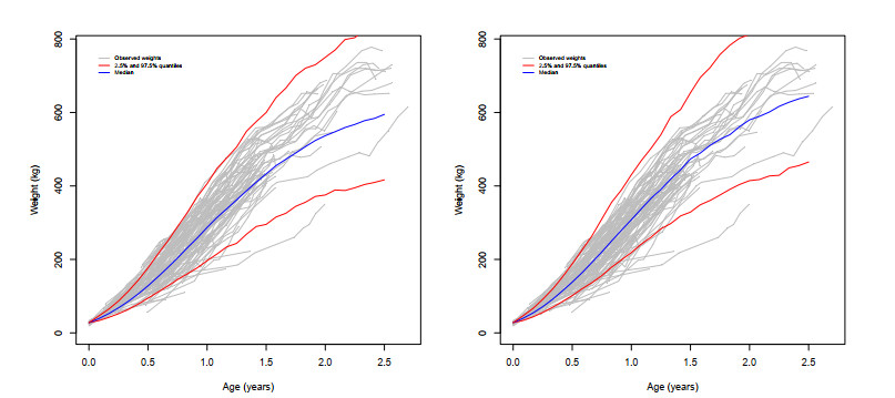
We used a class of stochastic differential equations (SDE) to model the evolution of cattle weight that, by an appropriate transformation of the weight, resulted in a variant of the Ornstein-Uhlenbeck model. In previous works, we have dealt with estimation, prediction, and optimization issues for this class of models. However, to incorporate individual characteristics of the animals, the average transformed size at maturity parameter $ \alpha $ and/or the growth parameter $ \beta $ may vary randomly from animal to animal, which results in SDE mixed models. Obtaining a closed-form expression for the likelihood function to apply the maximum likelihood estimation method is a difficult, sometimes impossible, task. We compared the known Laplace approximation method with the delta method to approximate the integrals involved in the likelihood function. These approaches were adapted to allow the estimation of the parameters even when the requirement of most existing methods, namely having the same age vector of observations for all trajectories, fails, as it did in our real data example. Simulation studies were also performed to assess the performance of these approximation methods. The results show that the approximation methods under study are a very good alternative for the estimation of SDE mixed models.
Citation: Nelson T. Jamba, Gonçalo Jacinto, Patrícia A. Filipe, Carlos A. Braumann. Estimation for stochastic differential equation mixed models using approximation methods[J]. AIMS Mathematics, 2024, 9(4): 7866-7894. doi: 10.3934/math.2024383
We used a class of stochastic differential equations (SDE) to model the evolution of cattle weight that, by an appropriate transformation of the weight, resulted in a variant of the Ornstein-Uhlenbeck model. In previous works, we have dealt with estimation, prediction, and optimization issues for this class of models. However, to incorporate individual characteristics of the animals, the average transformed size at maturity parameter $ \alpha $ and/or the growth parameter $ \beta $ may vary randomly from animal to animal, which results in SDE mixed models. Obtaining a closed-form expression for the likelihood function to apply the maximum likelihood estimation method is a difficult, sometimes impossible, task. We compared the known Laplace approximation method with the delta method to approximate the integrals involved in the likelihood function. These approaches were adapted to allow the estimation of the parameters even when the requirement of most existing methods, namely having the same age vector of observations for all trajectories, fails, as it did in our real data example. Simulation studies were also performed to assess the performance of these approximation methods. The results show that the approximation methods under study are a very good alternative for the estimation of SDE mixed models.

| [1] | P. A. Filipe, C. A. Braumann, N. M. Brites, C. J. Roquete, Prediction for individual growth in a random environment, in Recent Developments in Modeling and Applications in Statistics (eds. P. Oliveira, M. da Graça Temido, C. Henriques, M. Vichi), Springer, Berlin, Heidelberg, (2013), 193–201. https://doi.org/10.1007/978-3-642-32419-2_20 |
| [2] |
O. Garcia, A stochastic differential equation model for the height growth of forest stands, Biometrics, 39 (1983), 1059–1072. https://doi.org/10.2307/2531339 doi: 10.2307/2531339

|
| [3] |
N. T. Jamba, G. Jacinto, P. A. Filipe, C. A. Braumann, Likelihood function through the delta approximation in mixed sde models, Mathematics, 10 (2022). https://doi.org/10.3390/math10030385 doi: 10.3390/math10030385
|
| [4] |
O. Vasicek, An equilibrium characterization of the term structure, J. Financ. Econ., 5 (1977), 177–188. https://doi.org/10.1016/0304-405X(77)90016-2 doi: 10.1016/0304-405X(77)90016-2
|
| [5] |
P. A. Filipe, C. A. Braumann, N. M. Brites, C. J. Roquete, Modelling animal growth in random environments: an application using nonparametric estimation, Biometrical J., 52 (2010), 653–666. https://doi.org/10.1002/bimj.200900273 doi: 10.1002/bimj.200900273
|
| [6] |
P. A. Filipe, C. A. Braumann, C. J. Roquete, Multiphasic individual growth models in random environments, Methodol. Comput. Appl., 14 (2012), 49–56. https://doi.org/10.1007/s11009-010-9172-0 doi: 10.1007/s11009-010-9172-0
|
| [7] |
G. Jacinto, P. A. Filipe, C. A. Braumann, Profit optimization of cattle growth with variable prices, Methodol. Comput. Appl., 24 (2022a), 1917–1952. https://doi.org/10.1007/s11009-021-09889-z doi: 10.1007/s11009-021-09889-z
|
| [8] |
G. Jacinto, P. A. Filipe, C. A. Braumann, Weighted maximum likelihood estimation for individual growth models, Optimization, 71 (2022b), 3295–3311. https://doi.org/10.1080/02331934.2022.2075745 doi: 10.1080/02331934.2022.2075745
|
| [9] |
U. Picchini, S. Ditlevsen, Practical estimation of high dimensional stochastic differential mixed-effects models, Comput. Stat. Data An., 55 (2011), 1426–1444. https://doi.org/10.1016/j.csda.2010.10.003 doi: 10.1016/j.csda.2010.10.003
|
| [10] |
R. Wolfinger, Laplace's approximation for nonlinear mixed models, Biometrika, 80 (1993), 791–795. https://doi.org/10.2307/2336870 doi: 10.2307/2336870
|
| [11] |
M. Delattre, A review on asymptotic inference in stochastic differential equations with mixed effects, Jan. J. Stat. Data Sci., 4 (2021), 543–575. https://doi.org/10.1007/s42081-021-00105-3 doi: 10.1007/s42081-021-00105-3
|
| [12] |
I. Botha, R. Kohn, C. Drovandi, Particle methods for stochastic differential equation mixed effects models, Bayesian Anal., 16 (2021), 575–609. https://doi.org/10.1214/20-BA1216 doi: 10.1214/20-BA1216
|
| [13] |
S. Wiqvist, A. Golightly, A. T. McLean, U. Picchini, Efficient inference for stochastic differential equation mixed-effects models using correlated particle pseudo-marginal algorithms, Comput. Stat. Data Anal., 157 (2021), 107151. https://doi.org/10.1016/j.csda.2020.107151 doi: 10.1016/j.csda.2020.107151
|
| [14] |
M. G. Ruse, A. Samson, S. Ditlevsen, Inference for biomedical data by using diffusion models with covariates and mixed effects, J. Royal Stat. Soc. C-Appl., 69 (2020), 167–193. https://doi.org/10.1111/rssc.12386 doi: 10.1111/rssc.12386
|
| [15] |
R. V. Overgaard, N. Jonsson, C. W. Tornøe, H. Madsen, Non-linear mixed-effects models with stochastic differential equations: Implementation of an estimation algorithm, J. Pharmacokinet. Phar., 32 (2005), 85–107. https://doi.org/10.1007/s10928-005-2104-x doi: 10.1007/s10928-005-2104-x
|
| [16] | U. Picchini, A. D. Gaetano, S. Ditlevsen, Stochastic differential mixed-effects models, Scand. J. Stat., 37 (2010), 67–90. http://www.jstor.org/stable/41000916 |
| [17] | M. Delattre, C. Dion, Msdeparest: Parametric estimation in mixed-effects stochastic differential equations, R package version 1.7, (2017). https://CRAN.R-project.org/package = MsdeParEst |
| [18] | C. Dion, A. Samson, S. Hermann, mixedsde: Estimation methods for stochastic differential mixed effects models, R package version 5.0, (2018). https://CRAN.R-project.org/package = mixedsde |
| [19] |
S. Klim, S. B. Mortensen, N. R. Kristensen, R. V. Overgaard, H. Madsen, Population stochastic modelling (psm)-an r package for mixed-effects models based on stochastic differential equations. Comput. Meth. Prog. Bio., 94 (2009), 279–289. https://doi.org/10.1016/j.cmpb.2009.02.001 doi: 10.1016/j.cmpb.2009.02.001
|
| [20] |
M. Delattre, V. Genon-Catalot, A. Samson, Maximum likelihood estimation for stochastic differential equations with random effects, Scand. J. Stat., 40 (2013), 322–343. https://doi.org/10.1111/j.1467-9469.2012.00813.x doi: 10.1111/j.1467-9469.2012.00813.x
|
| [21] | C. A. Braumann, Introduction to Stochastic Differential Equations with Applications to Modelling in Biology and Finance, John Wiley & Sons, (2019). https://doi.org/10.1002/9781119166092 |
| [22] |
J. Leander, M. Jirstrand, U. G. Eriksson, R. Palmér, A stochastic mixed effects model to assess treatment effects and fluctuations in home-measured peak expiratory flow and the association with exacerbation risk in asthma, CPT: Pharmacomet. Syst., 11 (2022), 212–224. https://doi.org/10.1002/PSP4.12748 doi: 10.1002/PSP4.12748
|
| [23] |
K. Wang, L. Marciani, G. L. Amidon, D. E. Smith, D. Sun, Stochastic differential equation-based mixed effects model of the fluid volume in the fasted stomach in healthy adult human, AAPS J., 25 (2023), 76. https://doi.org/10.1208/s12248-023-00840-3 doi: 10.1208/s12248-023-00840-3
|
| [24] |
U. Picchini, S. Ditlevsen, A. De Gaetano, Maximum likelihood estimation of a time-inhomogeneous stochastic differential model of glucose dynamics, Math. Med. Biol., 25 (2008), 141–155. https://doi.org/10.1093/imammb/dqn011 doi: 10.1093/imammb/dqn011
|
| [25] | U. Picchini, Stochastic Differential Models with Applications to Physiology, PhD thesis, University of Rome, Rome, Italy, 2006. |
Figures(1) / Tables(8)

Nelson T. Jamba, Gonçalo Jacinto, Patrícia A. Filipe, Carlos A. Braumann. Estimation for stochastic differential equation mixed models using approximation methods[J]. AIMS Mathematics, 2024, 9(4): 7866-7894. doi: 10.3934/math.2024383


 DownLoad: