We studied the weekly number and the growth/decline rates of COVID-19 deaths of the period from October 31, 2022, to February 9, 2023, in Italy. We found that the COVID-19 winter wave reached its peak during the three holiday weeks from December 16, 2022, to January 5, 2023, and it was definitely trending downward, returning to the same number of deaths as the end of October 2022, in the first week February 2023. During this period of 15 weeks, that wave caused a number of deaths as large as 8,526. Its average growth rate was +7.89% deaths per week (10 weeks), while the average weekly decline rate was -15.85% (5 weeks). At the time of writing of this paper, Italy has been experiencing a new COVID-19 wave, with the latest 7 weekly bulletins (October 26, 2023 – December 13, 2023) showing that deaths have climbed from 148 to 322. The weekly growth rate had risen by +14.08% deaths, on average. Hypothesizing that this 2023/2024 wave will have a total duration similar to that of 2022/2023, with comparable extensions of both the growth period and the decline period and similar growth/decline rates, we predict that the number of COVID-19 deaths of the period from the end of October 2023 to the beginning of February 2024 should be less than 4100. A preliminary assessment of this forecast, based on 11 of the 15 weeks of the period, has already confirmed the accuracy of this approach.
Citation: Marco Roccetti. Drawing a parallel between the trend of confirmed COVID-19 deaths in the winters of 2022/2023 and 2023/2024 in Italy, with a prediction[J]. Mathematical Biosciences and Engineering, 2024, 21(3): 3742-3754. doi: 10.3934/mbe.2024165
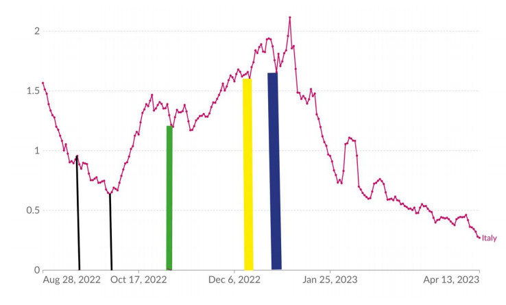
We studied the weekly number and the growth/decline rates of COVID-19 deaths of the period from October 31, 2022, to February 9, 2023, in Italy. We found that the COVID-19 winter wave reached its peak during the three holiday weeks from December 16, 2022, to January 5, 2023, and it was definitely trending downward, returning to the same number of deaths as the end of October 2022, in the first week February 2023. During this period of 15 weeks, that wave caused a number of deaths as large as 8,526. Its average growth rate was +7.89% deaths per week (10 weeks), while the average weekly decline rate was -15.85% (5 weeks). At the time of writing of this paper, Italy has been experiencing a new COVID-19 wave, with the latest 7 weekly bulletins (October 26, 2023 – December 13, 2023) showing that deaths have climbed from 148 to 322. The weekly growth rate had risen by +14.08% deaths, on average. Hypothesizing that this 2023/2024 wave will have a total duration similar to that of 2022/2023, with comparable extensions of both the growth period and the decline period and similar growth/decline rates, we predict that the number of COVID-19 deaths of the period from the end of October 2023 to the beginning of February 2024 should be less than 4100. A preliminary assessment of this forecast, based on 11 of the 15 weeks of the period, has already confirmed the accuracy of this approach.

| [1] |
L. Casini, M, Roccetti, Reopening Italy's schools in September 2020: A Bayesian estimation of the change in the growth rate of new SARSCoV-2 cases, BMJ Open, 11 (2021), 1–7. https://doi.org/10.1136/bmjopen-2021-051458 doi: 10.1136/bmjopen-2021-051458

|
| [2] |
C. Liu, J. Huang, S. Chen, D. Wang, L. Zhang, X. Liu, X. Lian, The impact of crowd gatherings on the spread of COVID-19, Environ. Res., 213 (2022), 1–8. https://doi.org/10.1016/j.envres.2022.113604 doi: 10.1016/j.envres.2022.113604
|
| [3] |
R. Cappi, L. Casini, D. Tosi, M. Roccetti. Questioning the seasonality of SARS-COV-2: A Fourier spectral analysis, BMJ Open, 12 (2022), 1–12. https://doi.org/10.1136/bmjopen-2022-061602 doi: 10.1136/bmjopen-2022-061602
|
| [4] | Italian Ministry of Health. Weekly Bulletins—COVID-19. Available from: https://www.salute.gov.it/portale/nuovocoronavirus/archivioBollettiniNuovoCoronavirus.jsp (accessed on 15 December 2023). |
| [5] | E. Mathieu, H. Ritchie, L. Rodés Guirao, C. Appel, D. Gavrilov, C. Giattino, et al., Coronavirus (COVID-19) Deaths, 2023. Available from: https://ourworldindata.org/covid-deaths (accessed on 15 December 2023). |
| [6] |
C. El Aoun, H. Eleuch, H. Ben Ayed, E. Aïmeur, F. Kamun, Analogy in Making Predictions, J. Decis. Syst., 16 (2007), 393–416. https://doi.org/10.3166/jds.16.393-416 doi: 10.3166/jds.16.393-416
|
| [7] |
M. Bar, The proactive brain: using analogies and associations to generate predictions, Trends Cogn. Sci., 11 (2007), 280–289. https://doi.org/10.1016/j.tics.2007.05.005 doi: 10.1016/j.tics.2007.05.005
|
| [8] |
I. Cooper, A. Mondal, C.G. Antonopoulos, A SIR model assumption for the spread of COVID-19 in different communities, Chaos Solit. Fractals, 139 (2020), 1–14. https://doi.org/10.1016/j.chaos.2020.110057 doi: 10.1016/j.chaos.2020.110057
|
| [9] |
M. Gaspari, The impact of test positivity on surveillance with asymptomatic carriers, Epidemiol. Methods, 11 (2022). https://doi.org/10.1515/em-2022-0125 doi: 10.1515/em-2022-0125
|
| [10] |
M. Roccetti, Excess mortality and COVID-19 deaths in Italy: A peak comparison study, Math. Biosci. Eng., 20 (2023), 7042–7055. https://doi.org/10.3934/mbe.2023304 doi: 10.3934/mbe.2023304
|
| [11] |
S. Piconi, S. Pontiggia, M. Franzetti, F. Branda, D.Tosi, Statistical models to predict clinical outcomes with anakinra vs. tocilizumab treatments for severe pneumonia in COVID19 patients, Eur. J. Intern. Med., 112 (2023), 118–120. https://doi.org/10.1016/j.ejim.2023.01.024 doi: 10.1016/j.ejim.2023.01.024
|
| [12] |
D. Tosi, A. Campi, How schools affected the COVID-19 pandemic in Italy: Data analysis for Lombardy Region, Campania Region and Emilia Region, Future Internet, 13 (2021), 1–12. https://doi.org/10.3390/fi13050109 doi: 10.3390/fi13050109
|
| [13] |
D. Tosi, A. Campi, How data analytics and Big Data can help scientists in managing COVID-19 diffusion: A model to predict the COVID-19 diffusion in Italy and Lombardy Region, J. Med. Internet Res., 22 (2020), 1–21, https://doi.org/10.2196/21081 doi: 10.2196/21081
|
| [14] |
D. Tosi, A. Verde, M. Verde, Clarification of misleading perceptions of COVID-19 fatality and testing rates in Italy: Data analysis, J. Med. Internet Res., 22 (2020), 1–14. https://doi.org/10.2196/19825 doi: 10.2196/19825
|
| [15] | Italian RAI Broadcaster, RAINews. Weekly Bullettins COVID-19. Available from: https://www.rainews.it/ran24/speciali/2020/covid19/ (accessed on 15 December 2023). |
| [16] |
K. C. Greene, S. Armstrong, J. Scott, Structured analogies for forecasting. Int. J. Forecast., 23 (2007), 365–376. https://doi.org/10.1016/j.ijforecast.2007.05.005 doi: 10.1016/j.ijforecast.2007.05.005
|
| [17] |
P. Nasa, R. Jain, D. Juneja, Delphi methodology in healthcare research: How to decide its appropriateness, World J. Methodol., 11 (2021), 116–129. https://doi.org/10.5662/wjm.v11.i4.116 doi: 10.5662/wjm.v11.i4.116
|
| [18] |
P. Salomoni, S. Mirri, S. Ferretti, M. Roccetti, Profiling learners with special needs for custom e-learning experiences, a closed case?, ACM Int. Conf. Proceed. Ser., 225 (2007), 84–92. https://doi.org/10.1145/1243441.1243462 doi: 10.1145/1243441.1243462
|
| [19] |
S-P. Jun, T-E. Sung, H-W Park, Forecasting by analogy using the web search traffic, Technol. Forecasting Soc. Change, 115 (2017), 37–51, https://doi.org/10.1016/j.techfore.2016.09.014 doi: 10.1016/j.techfore.2016.09.014
|
| [20] | Italian Ministry of Health. Vaccinations 2023/2024 – COVID-19. Available from: https://www.governo.it/it/cscovid19/report-vaccini/ (accessed on 15 December 2023). |
| [21] |
C. Mattiuzzi, G. Lippi, Update on the status of COVID-19 vaccination in Italy - April 2023. Immunol. Res., 71 (2023), 671–672. https://doi.org/10.1007/s12026-023-09383-3 doi: 10.1007/s12026-023-09383-3
|
| [22] | K. Katella, Omicron, Delta, Alpha, and More: What to know about the Coronavirus variants, Yale Medicine, 2023. Available from: https://www.yalemedicine.org/news/covid-19-variants-of-concern-omicron (accessed on 15 December 2023). |
| [23] |
F. Baum T. Freeman, C. Musolino, M. Abramovitz, W. De Ceukelaire, J. Flavel, et al., Explaining covid-19 performance: What factors might predict national responses? BMJ, 372 (2021). https://doi.org/10.1136/bmj.n91 doi: 10.1136/bmj.n91
|
| [24] |
I. Ciufolini, A. Paolozzi, An improved mathematical prediction of the time evolution of the Covid-19 pandemic in Italy, with a Monte Carlo simulation and error analyses, Eur. Phys. J. Plus, 135 (2020), 1–13. https://doi.org/10.1140/epjp/s13360-020-00488-4 doi: 10.1140/epjp/s13360-020-00488-4
|
| [25] | Italian Historical Video Archive - Istituto Luce. Flu Epidemic in Italy, 1969–1970. Available from: https://www.raiplay.it/video/2020/03/Frontiere---Coronavirus-Asiatica-del-1969-In-Italia-5000-morti-e-13-milioni-a-letto-d93814e9-3b14-4e5c-8b41-e0eaa87f7cd0.html (accessed on 15 December 2023). |
| [26] |
C. Rizzo, A. Bella, C. Viboud, L. Simonsen, M.A. Miller, M.C. Rota, et al., Trends for Influenza-related Deaths during Pandemic and Epidemic Seasons, Italy, 1969–2001, Emerg. Infect. Dis., 13 (2007), 694–699. https://doi.org/10.3201/eid1305.061309 doi: 10.3201/eid1305.061309
|
Figures(1) / Tables(2)

Marco Roccetti. Drawing a parallel between the trend of confirmed COVID-19 deaths in the winters of 2022/2023 and 2023/2024 in Italy, with a prediction[J]. Mathematical Biosciences and Engineering, 2024, 21(3): 3742-3754. doi: 10.3934/mbe.2024165


 DownLoad: