Laser marking on polymer composite surfaces can be difficult to read and cause readability problems for electronic decoding equipment on production lines due to poor interaction between the laser and the fibers used to reinforce these materials. This problem can be solved with the right choice of marking parameters, resulting in savings for companies by avoiding production problems such as rejection, scrap and customer complaints. The present work uses the polybutylene terephthalate/glass fiber (PBT/GF) composite used in the manufacture of instrument panels for motorcycles. The tests were carried out with different laser marking parameters using a neodymium:yttrium-aluminum-garnet (Nd:YAG) laser. Subsequently, the laser-marked data matrix codes (DMC) were analyzed using a microscope verifier to evaluate the quality according to the ISO/IEC 29158:2020 standard. A detailed analysis of these surfaces was also carried out to observe some physical and chemical changes using scanning electron microscopy (SEM) and energy dispersive X-ray spectroscopy (EDS). The optical analysis showed that lower radiation power and pulse frequency and higher marking speed corresponded to weaker laser marking and therefore poorer DMC code quality, which was confirmed by the SEM. EDS showed that the laser marking process did not cause the chemical changes on the sample surface.
Citation: R.C.M. Sales-Contini, J.P. Costa, F.J.G. Silva, A.G. Pinto, R.D.S.G. Campilho, I.M. Pinto, V.F.C. Sousa, R.P. Martinho. Influence of laser marking parameters on data matrix code quality on polybutylene terephthalate/glass fiber composite surface using microscopy and spectroscopy techniques[J]. AIMS Materials Science, 2024, 11(1): 150-172. doi: 10.3934/matersci.2024009
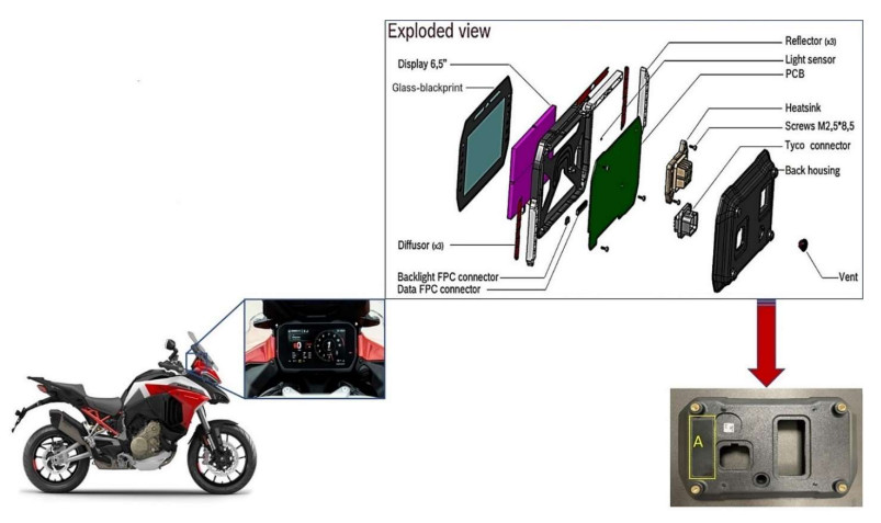
Laser marking on polymer composite surfaces can be difficult to read and cause readability problems for electronic decoding equipment on production lines due to poor interaction between the laser and the fibers used to reinforce these materials. This problem can be solved with the right choice of marking parameters, resulting in savings for companies by avoiding production problems such as rejection, scrap and customer complaints. The present work uses the polybutylene terephthalate/glass fiber (PBT/GF) composite used in the manufacture of instrument panels for motorcycles. The tests were carried out with different laser marking parameters using a neodymium:yttrium-aluminum-garnet (Nd:YAG) laser. Subsequently, the laser-marked data matrix codes (DMC) were analyzed using a microscope verifier to evaluate the quality according to the ISO/IEC 29158:2020 standard. A detailed analysis of these surfaces was also carried out to observe some physical and chemical changes using scanning electron microscopy (SEM) and energy dispersive X-ray spectroscopy (EDS). The optical analysis showed that lower radiation power and pulse frequency and higher marking speed corresponded to weaker laser marking and therefore poorer DMC code quality, which was confirmed by the SEM. EDS showed that the laser marking process did not cause the chemical changes on the sample surface.

| [1] |
Marin-Garcia JA, Pardo del Val M, Bonavía Martín T (2008) Longitudinal study of the results of continuous improvement in an industrial company. Team Perform Manag 14: 56–69. https://doi.org/10.1108/13527590810860203 doi: 10.1108/13527590810860203

|
| [2] |
Grütter AW, Field JM, Faull NHB (2002) Work team performance over time: Three case studies of South African manufacturers. J Oper Manag 20: 641–657. https://doi.org/10.1016/S0272-6963(02)00031-1 doi: 10.1016/S0272-6963(02)00031-1
|
| [3] | Bosch (2021) Good Service Practices Manual. BOSCH Internal release, Braga, Portugal. |
| [4] |
Barad M (2014) Design of experiments (DoE)—A valuable multi-purpose methodology. Appl Math 5: 2120–2129. https://doi.org/10.4236/am.2014.514206 doi: 10.4236/am.2014.514206
|
| [5] | Loh SH, The PC, Sim JJ, et al. (2023) Decoding dot peen data matrix code with deep learning capability for product traceability. AMS 7: 38–48. Available from: http://arqiipubl.com/ojs/index.php/AMS_Journal/article/view/385. |
| [6] |
Li C, Lu C, Li J (2018) Research on the quality of laser marked data matrix symbols. Key Eng Mater 764: 219–224. https://doi.org/10.1088/1757-899X/380/1/012023 doi: 10.1088/1757-899X/380/1/012023
|
| [7] |
Sobotova L, Demec P (2015) Laser marking of metal materials. MM Sci J 12: 808–812. https://doi.org/10.17973/MMSJ.2015_12_201410 doi: 10.17973/MMSJ.2015_12_201410
|
| [8] | Javale V, Nair VA (2013) Review on laser marking by Nd-Yag laser and fiber laser. Int J Sci Res Dev 1: 1995–1997. Available from: https://ijsrd.com/Article.php?manuscript = IJSRDV1I9075. |
| [9] | Trotec Laser (2019) Laser handbook: A comprehensive guide to industrial laser applications, Austria: Trotec Laser. |
| [10] |
Qi J, Wang K, Zhu Y (2003) A study on the laser marking process of stainless steel. J Mater Process Technol 139: 273–276. https://doi.org/10.1016/S0924-0136(03)00234-6 doi: 10.1016/S0924-0136(03)00234-6
|
| [11] |
Jangsombatsiri W, Porter JD (2007) Laser direct-part marking of data matrix symbols on carbon steel substrates. J Manuf Sci E-T ASME 129: 583–591. https://doi.org/10.1115/1.2716704 doi: 10.1115/1.2716704
|
| [12] |
Zelenska KS, Zelensky SE, Poperenko LV, et al. (2016) Thermal mechanisms of laser marking in transparent polymers with light-absorbing microparticles. Opt Laser Technol 76: 96–100. https://doi.org/10.1016/j.optlastec.2015.07.011 doi: 10.1016/j.optlastec.2015.07.011
|
| [13] |
Czyzewski P, Sykutera D, Rojewski M (2022) The impact of selected laser-marking parameters and surface conditions on white polypropylene moldings. Polymer 14: 1879. https://doi.org/10.3390/polym14091879 doi: 10.3390/polym14091879
|
| [14] | Lu G, Wu Y, Zhang Y, et al. (2020) Surface laser-marking and mechanical properties of acrylonitrile-butadiene-styrene copolymer composites with organically modified montmorillonite. ACS Omega 5: 19255-19267. https://dx.doi.org/10.1021/acsomega.0c02803 |
| [15] | Narica P, Fedotovs J (2019) Marking of a small-sized QR code on a plastic surface. 19th International Conference on Reliability and Statistics in Transportation and Communication, Riga, Latvia Springer, 16–19. https://link.springer.com/chapter/10.1007/978-3-030-44610-9_41 |
| [16] | Li WH (2021) Preparation of laser markable polyamide compounds. 2nd International Conference on Graphene and Novel Nanomaterials (GNN), 1765: 1–5. https://doi.org/10.1088/1742-6596/1765/1/012003 |
| [17] |
Chen MF, Hsiao WT, Huang WL, et al. (2009) Laser coding on the eggshell using pulsed laser marking system. J Mater Process Technol 209: 737–744. https://doi.org/10.1016/j.jmatprotec.2008.02.075 doi: 10.1016/j.jmatprotec.2008.02.075
|
| [18] |
Cheng J, Zhou J, Zhang C, et al. (2019) Enhanced laser marking of polypropylene induced by "core-shell" ATO@PI laser-sensitive composite. Polym Degrad Stabil 167: 77–85. https://doi.org/10.1016/j.polymdegradstab.2019.06.022 doi: 10.1016/j.polymdegradstab.2019.06.022
|
| [19] |
Yang J, Xiang M, Zhu Y, et al. (2023) Influences of carbon nanotubes/polycarbonate composite on enhanced local laser marking properties of polypropylene. Polym Bull 80: 1321–1333. https://doi.org/10.1007/s00289-022-04123-3 doi: 10.1007/s00289-022-04123-3
|
| [20] |
Zhong W, Cao Z, Qiu P, et al. (2015) Laser-marking mechanism of thermoplastic polyurethane/Bi2O3 composites. ACS Appl Mater Interface 7: 24142-24149. https://doi.org/10.1021/acsami.5b07406 doi: 10.1021/acsami.5b07406
|
| [21] |
Cao Z, Hu Y, Lu Y, et al. (2017) Laser-induced blackening on surfaces of thermoplastic polyurethane/BiOCl composites. Polym Degrad Stabil 141: 33–40. http://dx.doi.org/10.1016/j.polymdegradstab.2017.05.004 doi: 10.1016/j.polymdegradstab.2017.05.004
|
| [22] |
Ng TW, Yeo SC (2000) Aesthetic laser marking assessment. Opt Laser Technol 32: 187–191. https://doi.org/10.1016/S0030-3992(00)00040-2 doi: 10.1016/S0030-3992(00)00040-2
|
| [23] |
Ng TW, Yeo SC (2001) Aesthetic laser marking assessment using luminance ratios. Opt Laser Eng 35: 177–186. https://doi.org/10.1016/S0143-8166(01)00005-7 doi: 10.1016/S0143-8166(01)00005-7
|
| [24] |
Arai S, Tsunoda S, Yamaguchi A, et al. (2019) Effect of anisotropy in the build direction and laser-scanning conditions on characterization of short-glass-fiber-reinforced PBT for laser sintering. Opt Laser Technol 113: 345–356. https://doi.org/10.1016/j.optlastec.2019.01.012 doi: 10.1016/j.optlastec.2019.01.012
|
| [25] |
Greiner S, Wudy K, Lanzl L, et al. (2017) Selective laser sintering of polymer blends: Bulk properties and process behaviour. Polym Test 64: 136–144. https://doi.org/10.1016/j.polymertesting.2017.09.039 doi: 10.1016/j.polymertesting.2017.09.039
|
| [26] |
Silva LRR, Marques EAS, Carbas RJC, et al. (2002) Study of the optical, thermal, morphological and mechanical characteristics of a laser weldable fibre reinforced polymer. Polym Compos 43: 4038–4055. https://doi.org/10.1002/pc.26677 doi: 10.1002/pc.26677
|
| [27] |
Ng TW, Yeo SC (2000) Aesthetic laser marking assessment using spectrophotometers. J Mater Process Technol 104: 280–283. https://doi.org/10.1016/S0924-0136(00)00548-3 doi: 10.1016/S0924-0136(00)00548-3
|
| [28] | BASF (2023) Product Data Sheet Ultradur B 4406 G6 05/2023 PBT-GF30 FR(17). Available from: https://www.basf.com/cn/documents/en/chinaplas/Ultradur_brochure.pdf. |
| [29] | ISO/IEC 29158 (2020) Information technology—Automatic identification and data capture techniques-Direct Part Mark (DPM) Quality Guideline. |
| [30] | Bociga E, Jaruga T (2007) Experimental investigation of polymer flow in injection mould. Arch Mater Sci Eng 28: 165–172. |
| [31] |
Wang G, Zhao G, Wang X (2013) Effects of cavity surface temperature on reinforced plastic part surface appearance in rapid heat cycle moulding. Mater Design 44: 509–520. https://doi.org/10.1016/j.matdes.2012.08.039 doi: 10.1016/j.matdes.2012.08.039
|
| [32] |
Gim J, Turng LS (2022) A review of current advancements in high surface quality injection moulding: Measurement, influencing factors, prediction, and control. Polym Test 115: 107718. https://doi.org/10.1016/j.polymertesting.2022.107718 doi: 10.1016/j.polymertesting.2022.107718
|
| [33] |
Uysal S, Mercan M, Uzun L (2020) Serial number restoration on polymer surfaces: A survey of recent literature. Forensic Chem 20: 100267. https://doi.org/10.1016/j.forc.2020.100267 doi: 10.1016/j.forc.2020.100267
|
| [34] |
Katterwe H (1994) The recovery of erased numbers in polymers. J Forensic Sci Soc 34: 11–16. https://doi.org/10.1016/S0015-7368(94)72876-0 doi: 10.1016/S0015-7368(94)72876-0
|
| [35] | Young RJ, Lovell PA (2011) Introduction to Polymers, 3 Eds., Boca Raton: CRC Press. https://doi.org/10.1201/9781439894156 |
| [36] | Aly AA (2015) Heat treatment of polymers: A review. Int J Mater Chem Phys 1: 132–140. https://api.semanticscholar.org/CorpusID: 53342231 |
| [37] |
Pieretti EF, Costa I (2013) Surface characterization of ASTM F139 stainless steel marked by laser and mechanical techniques. Electrochim Acta 114: 838–843. https://doi.org/10.1016/j.electacta.2013.05.101 doi: 10.1016/j.electacta.2013.05.101
|
| [38] | Lu G, Wu Y, Zhang Y, et al. (2020) Surface laser-marking and mechanical properties of acrylonitrile butadiene-styrene copolymer composites with organically modified montmorillonite. ACS Omega 5: 19255-19267. https://doi.org/10.1021/acsomega.0c02803 |
| [39] |
Man HC, Li M, Yue TM (1998) Surface treatment of thermoplastic composites with an excimer laser. Int J Adhes Adhes 18: 151–157. https://doi.org/10.1016/S0143-7496(97)00044-4 doi: 10.1016/S0143-7496(97)00044-4
|
| [40] |
Cao Z, Hu Y, Yu Q, et al (2017) Facile fabrication, structures, and properties of laser-marked polyacrylamide/Bi2O3 hydrogels. Adv Eng Mater 19: 1600826. https://doi.org/10.1002/adem.201600826 doi: 10.1002/adem.201600826
|
| [41] |
Obilor AF, Pacella M, Wilson A, et al. (2022) Micro-texturing of polymer surfaces using lasers: A review. Int J Adv Manuf Technol 120: 103–135. https://doi.org/10.1007/s00170-022-08731-1 doi: 10.1007/s00170-022-08731-1
|
| [42] | Margolis JM (2006) Engineering Plastic Handbook, 1 Ed., New York: McGraw-Hill Professional. https://doi.org/10.1036/0071457674 |
| [43] |
Cheng J, Li H, Zhou J, et al. (2018) Influences of diantimony trioxide on laser-marking properties of thermoplastic polyurethane. Polym Degrad Stabil 154: 149–156. https://doi.org/10.1016/j.polymdegradstab.2018.05.031 doi: 10.1016/j.polymdegradstab.2018.05.031
|


Figures(10) / Tables(3)

R.C.M. Sales-Contini, J.P. Costa, F.J.G. Silva, A.G. Pinto, R.D.S.G. Campilho, I.M. Pinto, V.F.C. Sousa, R.P. Martinho. Influence of laser marking parameters on data matrix code quality on polybutylene terephthalate/glass fiber composite surface using microscopy and spectroscopy techniques[J]. AIMS Materials Science, 2024, 11(1): 150-172. doi: 10.3934/matersci.2024009


 DownLoad: