Encouraged by the tremendous success of lithium iron phosphate (LiFePO4), analogous NaFePO4 has been predicted to show identical properties as LiFePO4. Synthesis of NaFePO4 materials in the maricite phase has been carried out using the sol-gel method with variations of calcination temperature and starting materials as sources of sodium Na2CO3 and NaCl. The resulted NaFePO4 maricite phase with the purity between 40% and 85%, according to X-ray diffractometry (XRD) characterization was obtained. The morphology and grain size of the particles in samples, as observed by a scanning electron microscope (SEM), tend to enlarge upon calcination at higher temperatures. The increment of calcination temperature increases the NaFePO4 maricite phase content in the sample. The impedance data analysis shows that the diffusion coefficient of Na+ ions and the electrical conductivity of a sample using Na2CO3 is higher than that of NaCl. This comprehensive study provides a feasible method and opens new opportunities for the continuous study of Na-ion batteries.
Citation: Fahmi Astuti, Rima Feisy Azmi, Mohammad Arrafi Azhar, Fani Rahayu Hidayah Rayanisaputri, Muhammad Redo Ramadhan, Malik Anjelh Baqiya, Darminto. Employing Na2CO3 and NaCl as sources of sodium in NaFePO4 cathode: A comparative study on structure and electrochemical properties[J]. AIMS Materials Science, 2024, 11(1): 102-113. doi: 10.3934/matersci.2024006
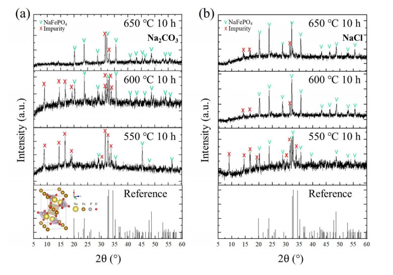
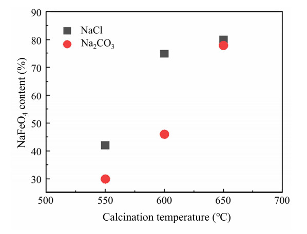
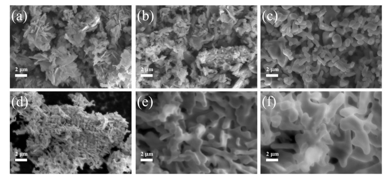
Encouraged by the tremendous success of lithium iron phosphate (LiFePO4), analogous NaFePO4 has been predicted to show identical properties as LiFePO4. Synthesis of NaFePO4 materials in the maricite phase has been carried out using the sol-gel method with variations of calcination temperature and starting materials as sources of sodium Na2CO3 and NaCl. The resulted NaFePO4 maricite phase with the purity between 40% and 85%, according to X-ray diffractometry (XRD) characterization was obtained. The morphology and grain size of the particles in samples, as observed by a scanning electron microscope (SEM), tend to enlarge upon calcination at higher temperatures. The increment of calcination temperature increases the NaFePO4 maricite phase content in the sample. The impedance data analysis shows that the diffusion coefficient of Na+ ions and the electrical conductivity of a sample using Na2CO3 is higher than that of NaCl. This comprehensive study provides a feasible method and opens new opportunities for the continuous study of Na-ion batteries.

| [1] |
Garcia LV, Ho YC, Thant MMM, et al. (2023) Lithium in a sustainable circular economy: A comprehensive review. Processes 11: 418. https://doi.org/10.3390/pr11020418 doi: 10.3390/pr11020418

|
| [2] |
Greim P, Solomon A, Breyer C (2020) Assessment of lithium criticality in the global energy transition and addressing policy gaps in transportation. Nat Commun 11: 4570. https://doi.org/10.1038/s41467-020-18402-y doi: 10.1038/s41467-020-18402-y
|
| [3] |
Liu M, Zhang P, Qu Z, et al. (2019) Conductive carbon nanofiber interpenetrated graphene architecture for ultra-stable sodium ion battery. Nat Commun 10: 3917. https://doi.org/10.1038/s41467-019-11925-z doi: 10.1038/s41467-019-11925-z
|
| [4] |
Sonoc A, Jeswiet J (2014) A review of lithium supply and demand and a preliminary investigation of a room temperature method to recycle lithium ion batteries to recover lithium and other materials. Procedia CIRP 15: 289–293. https://doi.org/10.1016/j.procir.2014.06.006 doi: 10.1016/j.procir.2014.06.006
|
| [5] |
Abraham KM (2020) How comparable are sodium-ion batteries to lithium-ion counterparts? ACS Energy Lett 5: 3544–3547. https://doi.org/10.1021/acsenergylett.0c02181 doi: 10.1021/acsenergylett.0c02181
|
| [6] |
Buonomenna MG, Bae J (2017) Sodium-ion batteries: A realistic alternative to lithium-ion batteries? Nanosci Nanotechnol-Asia 7: 139–154. https://doi.org/10.2174/2210681206666161019145001 doi: 10.2174/2210681206666161019145001
|
| [7] |
Yadav P, Patrike A, Wasnik K, et al. (2023) Strategies and practical approaches for stable and high energy density sodium-ion battery: A step closer to commercialization. Mater Today Sustain 22: 100385. https://doi.org/10.1016/j.mtsust.2023.100385 doi: 10.1016/j.mtsust.2023.100385
|
| [8] |
Xu G, Amine R, Abouimrane A, et al. (2018) Challenges in developing electrodes, electrolytes, and diagnostics tools to understand and advance sodium-ion batteries. Adv Energy Mater 8: 1702403. https://doi.org/10.1002/aenm.201702403 doi: 10.1002/aenm.201702403
|
| [9] |
Nayak PK, Yang L, Brehm W, et al. (2018) From lithium-ion to sodium-ion batteries: Advantages, challenges, and surprises. Angew Chem Int Ed 57: 102–120. https://doi.org/10.1002/anie.201703772 doi: 10.1002/anie.201703772
|
| [10] |
Fang Y, Liu Q, Xiao L, et al. (2015) High-performance olivine NaFePO4 microsphere cathode synthesized by aqueous electrochemical displacement method for sodium ion batteries. ACS Appl Mater Interfaces 7: 17977–17984. https://doi.org/10.1021/acsami.5b04691 doi: 10.1021/acsami.5b04691
|
| [11] |
Zhao A, Liu C, Ji F, et al. (2023) Revealing the phase evolution in Na4FexP4O12+x (2 ≤ x ≤ 4) cathode materials. ACS Energy Lett 8: 753–761. https://doi.org/10.1021/acsenergylett.2c02693 doi: 10.1021/acsenergylett.2c02693
|
| [12] |
Clément RJ, Billaud J, Armstrong AR, et al. (2016) Structurally stable Mg-doped P2-Na2/3Mn1−yMgyO2 sodium-ion battery cathodes with high rate performance: Insights from electrochemical, NMR and diffraction studies. Energy Environ Sci 9: 3240–3251. https://doi.org/10.1039/c6ee01750a doi: 10.1039/c6ee01750a
|
| [13] |
Hasa I, Passerini S, Hassoun J (2017) Toward high energy density cathode materials for sodium-ion batteries: Investigating the beneficial effect of aluminum doping on the P2-type structure. J Mater Chem A 5: 4467–4477. https://doi.org/10.1039/c6ta08667e doi: 10.1039/c6ta08667e
|
| [14] |
Shi Q, Qi R, Feng X, et al. (2022) Niobium-doped layered cathode material for high-power and low-temperature sodium-ion batteries. Nat Commun 13: 3205. https://doi.org/10.1038/s41467-022-30942-z doi: 10.1038/s41467-022-30942-z
|
| [15] |
Wang J, Fu C, Li Y, et al. (2022) Explore the effect of co doping on P2-Na0.67MnO2 prepared by hydrothermal method as cathode materials for sodium ion batteries. J Alloys Compd 918: 165569. https://doi.org/10.1016/j.jallcom.2022.165569 doi: 10.1016/j.jallcom.2022.165569
|
| [16] |
Avdeev M, Mohamed Z, Ling CD, et al. (2013) Magnetic structures of NaFePO4 maricite and triphylite polymorphs for sodium-ion batteries. Inorg Chem 52: 8685–8693. https://doi.org/10.1021/ic400870x doi: 10.1021/ic400870x
|
| [17] |
Hwang J, Matsumoto K, Nohira T, et al. (2017) Electrochemical sodiation-desodiation of maricite NaFePO4 in ionic liquid electrolyte. Electrochemistry 85: 675–679. https://doi.org/10.5796/electrochemistry.85.675 doi: 10.5796/electrochemistry.85.675
|
| [18] |
Zheng M, Bai Z, He Y, et al. (2020) Anionic redox processes in maricite- and triphylite-NaFePO4 of sodium-ion batteries. ACS Omega 5: 5192–5201. https://doi.org/10.1021/acsomega.9b04213 doi: 10.1021/acsomega.9b04213
|
| [19] |
Heubner C, Heiden S, Schneider M, et al. (2017) In-situ preparation and electrochemical characterization of submicron sized NaFePO4 cathode material for sodium-ion batteries. Electrochim Acta 233: 78–84. https://doi.org/10.1016/j.electacta.2017.02.107 doi: 10.1016/j.electacta.2017.02.107
|
| [20] |
Kundu D, Talaie E, Duffort V, et al. (2015) The emerging chemistry of sodium ion batteries for electrochemical energy Storage. Angew Chem Int Ed 54: 3431–3448. https://doi.org/10.1002/anie.201410376 doi: 10.1002/anie.201410376
|
| [21] |
Liu H, Li C, Zhang H, et al. (2006) Kinetic study on LiFePO4/C nanocomposites synthesized by solid state technique. J Power Sources 159: 717–720. https://doi.org/10.1016/j.jpowsour.2005.10.098 doi: 10.1016/j.jpowsour.2005.10.098
|
| [22] |
Wang D, Wu Y, Lv J, et al. (2019) Carbon encapsulated maricite NaFePO4 nanoparticles as cathode material for sodium-ion batteries. Colloid Surface A 583: 123957. https://doi.org/10.1016/j.colsurfa.2019.123957 doi: 10.1016/j.colsurfa.2019.123957
|
| [23] |
Zhu Y, Xu H, Ma J, et al. (2023) The recent advances of NASICON-Na3V2(PO4)3 cathode materials for sodium-ion batteries. J Solid State Chem 317: 123669. https://doi.org/10.1016/j.jssc.2022.123669 doi: 10.1016/j.jssc.2022.123669
|
| [24] |
Xia X, Cao Y, Liu Y, et al. (2019) MCNT-reinforced Na3Fe2(PO4)3 as cathode material for sodium-ion batteries. Arab J Sci Eng 45: 143–151. https://doi.org/10.1007/s13369-019-03979-4 doi: 10.1007/s13369-019-03979-4
|
| [25] |
Sun A, Beck FR, Haynes D, et al. (2012) Synthesis, characterization, and electrochemical studies of chemically synthesized NaFePO4. Mater Sci Eng B 177: 1729–1733. https://doi.org/10.1016/j.mseb.2012.08.004 doi: 10.1016/j.mseb.2012.08.004
|
| [26] |
Hwang J, Matsumoto K, Nohira T, et al. (2017) Electrochemical sodiation-desodiation of maricite NaFePO4 in ionic liquid electrolyte. Electrochemistry 85: 675–679. https://doi.org/10.5796/electrochemistry.85.675 doi: 10.5796/electrochemistry.85.675
|
| [27] |
Yu F, Wang Y, Guo C, et al. (2022) Spinel LiMn2O4 cathode materials in wide voltage window: Single-crystalline versus polycrystalline. Crystals 12: 317. https://doi.org/10.3390/cryst12030317 doi: 10.3390/cryst12030317
|
| [28] |
Kim T, Choi W, Shin H, et al. (2020) Applications of voltammetry in lithium ion battery research. J Electrochem Sci Technol 11: 14–25. https://doi.org/10.33961/jecst.2019.00619 doi: 10.33961/jecst.2019.00619
|
| [29] |
Ou J, Yang L, Jin F, et al. (2020) High performance of LiFePO4 with nitrogen-doped carbon layers for lithium ion batteries. Adv Powder Technol 31: 1220–1228. https://doi.org/10.1016/j.apt.2019.12.044 doi: 10.1016/j.apt.2019.12.044
|
| [30] |
Massaro A, Avila J, Goloviznina K, et al. (2020) Sodium diffusion in ionic liquid-based electrolytes for Na-ion batteries: the effect of polarizable force fields. Phys Chem Chem Phys 22: 20114–20122. https://doi.org/10.1039/d0cp02760j doi: 10.1039/d0cp02760j
|
| [31] |
Liu H, Li C, Zhang H, et al. (2006) Kinetic study on LiFePO4/C nanocomposites synthesized by solid state technique. J Power Sources 159: 717–720. https://doi.org/10.1016/j.jpowsour.2005.10.098 doi: 10.1016/j.jpowsour.2005.10.098
|
| [32] |
Astuti F, Miyajima M, Fukuda T, et al. (2019) Anionogenic magnetism combined with lattice symmetry in alkali-metal superoxide RbO2. J Phys Soc Jpn 88: 043701. https://doi.org/10.7566/jpsj.88.043701 doi: 10.7566/jpsj.88.043701
|
| [33] |
Kumar D, Kuo CN, Astuti F, et al. (2018) Nodeless superconductivity in the cage-type superconductor Sc5Ru6Sn18 with preserved time-reversal symmetry. J Phys: Condens Matter 30: 315803. https://doi.org/10.1088/1361-648x/aacf65 doi: 10.1088/1361-648x/aacf65
|
| [34] |
Månsson M, Nozaki H, Wikberg JM, et al. (2014) Lithium diffusion & magnetism in battery cathode material LixNi1/3CO1/3MN1/3O2. J Phys Conf Ser 551: 012037. https://doi.org/10.1088/1742-6596/551/1/012037 doi: 10.1088/1742-6596/551/1/012037
|
| [35] |
McClelland I, Johnston B, Baker PJ, et al. (2020) Muon spectroscopy for investigating diffusion in energy storage materials. Annu Rev Mater Res 50: 371–393. https://doi.org/10.1146/annurev-matsci-110519-110507 doi: 10.1146/annurev-matsci-110519-110507
|
| [36] |
Amores M, Baker PJ, Cussen EJ, et al. (2018) Na1.5La1.5TeO6: Na+ conduction in a novel Na-rich double perovskite. Chem Commun 54: 10040–10043. https://doi.org/10.1039/c8cc03367f doi: 10.1039/c8cc03367f
|
| [37] |
Månsson M, Sugiyama J (2013) Muon-spin relaxation study on Li- and Na-diffusion in solids. Phys Scripta 88: 068509. https://doi.org/10.1088/0031-8949/88/06/068509 doi: 10.1088/0031-8949/88/06/068509
|
| [38] |
Umegaki I, Nozaki H, Harada M, et al. (2018) Na diffusion in quasi one-dimensional ion conductor NaMn2O4 observed by μ+SR. JPS Conf Proc 21: 011018. https://doi.org/10.7566/jpscp.21.011018 doi: 10.7566/jpscp.21.011018
|
| [39] |
Bruce PG, Nowiński J, Gibson VC (1992) Temperature dependence of sodium ion diffusion in NaxWO2Cl2. Solid State Ionics 50: 41–45. https://doi.org/10.1016/0167-2738(92)90034-m doi: 10.1016/0167-2738(92)90034-m
|
| [40] |
Zhu Z, Chu I, Deng Z, et al. (2015) Role of Na+ interstitials and dopants in enhancing the Na+ conductivity of the cubic Na3PS4 superionic conductor. Chem Mater 27: 8318–8325. https://doi.org/10.1021/acs.chemmater.5b03656 doi: 10.1021/acs.chemmater.5b03656
|
| [41] |
Altundag S, Altin S, Yasar S, et al. (2023) Improved performance of the NaFePO4/hardcarbon sodium-ion full cell. Vacuum 210: 111853. https://doi.org/10.1016/j.vacuum.2023.111853 doi: 10.1016/j.vacuum.2023.111853
|
| [42] |
Sugiyama J, Nozaki H, Harada M, et al. (2011) Magnetic and diffusive nature of LiFePO4 investigated by muon spin rotation and relaxation. Phys Rev B 84: 054430. https://doi.org/10.1103/physrevb.84.054430 doi: 10.1103/physrevb.84.054430
|
Figures(6)

Fahmi Astuti, Rima Feisy Azmi, Mohammad Arrafi Azhar, Fani Rahayu Hidayah Rayanisaputri, Muhammad Redo Ramadhan, Malik Anjelh Baqiya, Darminto. Employing Na2CO3 and NaCl as sources of sodium in NaFePO4 cathode: A comparative study on structure and electrochemical properties[J]. AIMS Materials Science, 2024, 11(1): 102-113. doi: 10.3934/matersci.2024006


 DownLoad: