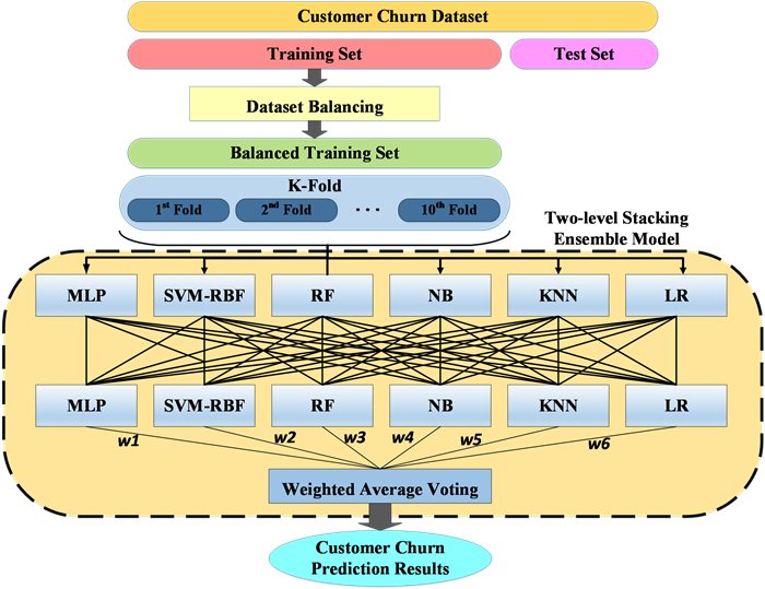
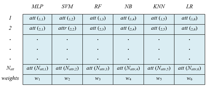
In today's competitive market, predicting clients' behavior is crucial for businesses to meet their needs and prevent them from being attracted by competitors. This is especially important in industries like telecommunications, where the cost of acquiring new customers exceeds retaining existing ones. To achieve this, companies employ Customer Churn Prediction approaches to identify potential customer attrition and develop retention plans. Machine learning models are highly effective in identifying such customers; however, there is a need for more effective techniques to handle class imbalance in churn datasets and enhance prediction accuracy in complex churn prediction datasets. To address these challenges, we propose a novel two-level stacking-mode ensemble learning model that utilizes the Whale Optimization Algorithm for feature selection and hyper-parameter optimization. We also introduce a method combining K-member clustering and Whale Optimization to effectively handle class imbalance in churn datasets. Extensive experiments conducted on well-known datasets, along with comparisons to other machine learning models and existing churn prediction methods, demonstrate the superiority of the proposed approach.
Citation: Bijan Moradi, Mehran Khalaj, Ali Taghizadeh Herat, Asghar Darigh, Alireza Tamjid Yamcholo. A swarm intelligence-based ensemble learning model for optimizing customer churn prediction in the telecommunications sector[J]. AIMS Mathematics, 2024, 9(2): 2781-2807. doi: 10.3934/math.2024138
In today's competitive market, predicting clients' behavior is crucial for businesses to meet their needs and prevent them from being attracted by competitors. This is especially important in industries like telecommunications, where the cost of acquiring new customers exceeds retaining existing ones. To achieve this, companies employ Customer Churn Prediction approaches to identify potential customer attrition and develop retention plans. Machine learning models are highly effective in identifying such customers; however, there is a need for more effective techniques to handle class imbalance in churn datasets and enhance prediction accuracy in complex churn prediction datasets. To address these challenges, we propose a novel two-level stacking-mode ensemble learning model that utilizes the Whale Optimization Algorithm for feature selection and hyper-parameter optimization. We also introduce a method combining K-member clustering and Whale Optimization to effectively handle class imbalance in churn datasets. Extensive experiments conducted on well-known datasets, along with comparisons to other machine learning models and existing churn prediction methods, demonstrate the superiority of the proposed approach.

| [1] | J. Wu, A study on customer acquisition cost and customer retention cost: Review and outlook, Proceedings of the 9th International Conference on Innovation & Management, 2012,799–803. |
| [2] |
A. Bilal Zorić, Predicting customer churn in banking industry using neural networks, INDECS, 14 (2016), 116–124. https://doi.org/10.7906/indecs.14.2.1 doi: 10.7906/indecs.14.2.1

|
| [3] |
K. G. M. Karvana, S. Yazid, A. Syalim, P. Mursanto, Customer churn analysis and prediction using data mining models in banking industry, 2019 International Workshop on Big Data and Information Security (IWBIS), 2019, 33–38. https://doi.org/10.1109/IWBIS.2019.8935884 doi: 10.1109/IWBIS.2019.8935884
|
| [4] |
A. Keramati, H. Ghaneei, S. M. Mirmohammadi, Developing a prediction model for customer churn from electronic banking services using data mining, Financ. Innov., 2 (2016), 10. https://doi.org/10.1186/s40854-016-0029-6 doi: 10.1186/s40854-016-0029-6
|
| [5] |
J. Kaur, V. Arora, S. Bali, Influence of technological advances and change in marketing strategies using analytics in retail industry, Int. J. Syst. Assur. Eng. Manag., 11 (2020), 953–961. https://doi.org/10.1007/s13198-020-01023-5 doi: 10.1007/s13198-020-01023-5
|
| [6] |
O. F. Seymen, O. Dogan, A. Hiziroglu, Customer churn prediction using deep learning, Proceedings of the 12th International Conference on Soft Computing and Pattern Recognition (SoCPaR 2020), 2020,520–529. https://doi.org/10.1007/978-3-030-73689-7_50 doi: 10.1007/978-3-030-73689-7_50
|
| [7] |
A. Dingli, V. Marmara, N. S. Fournier, Comparison of deep learning algorithms to predict customer churn within a local retail industry, Int. J. Mach. Learn. Comput., 7 (2017), 128–132. https://doi.org/10.18178/ijmlc.2017.7.5.634 doi: 10.18178/ijmlc.2017.7.5.634
|
| [8] |
M. C. Mozer, R. Wolniewicz, D. B. Grimes, E. Johnson, H. Kaushansky, Predicting subscriber dissatisfaction and improving retention in the wireless telecommunications industry, IEEE T. Neural Networks, 11 (2000), 690–696. https://doi.org/10.1109/72.846740 doi: 10.1109/72.846740
|
| [9] |
J. Hadden, A. Tiwari, R. Roy, D. Ruta, Computer assisted customer churn management: State-of-the-art and future trends, Comput. Oper. Res., 34 (2007), 2902–2917. https://doi.org/10.1016/j.cor.2005.11.007 doi: 10.1016/j.cor.2005.11.007
|
| [10] |
K. Coussement, D. Van den Poel, Churn prediction in subscription services: An application of support vector machines while comparing two parameter-selection techniques, Expert Syst. Appl., 34 (2008), 313–327. https://doi.org/10.1016/j.eswa.2006.09.038 doi: 10.1016/j.eswa.2006.09.038
|
| [11] |
J. Burez, D. Van den Poel, Handling class imbalance in customer churn prediction, Expert Syst. Appl., 36 (2009), 4626–4636. https://doi.org/10.1016/j.eswa.2008.05.027 doi: 10.1016/j.eswa.2008.05.027
|
| [12] |
P. C. Pendharkar, Genetic algorithm based neural network approaches for predicting churn in cellular wireless network services, Expert Syst. Appl., 36 (2009), 6714–6720. https://doi.org/10.1016/j.eswa.2008.08.050 doi: 10.1016/j.eswa.2008.08.050
|
| [13] |
A. Idris, A. Khan, Y. S. Lee, Genetic programming and adaboosting based churn prediction for telecom, IEEE international conference on Systems, Man, and Cybernetics (SMC), 2012, 1328–1332. https://doi.org/10.1109/ICSMC.2012.6377917 doi: 10.1109/ICSMC.2012.6377917
|
| [14] |
T. Vafeiadis, K. I. Diamantaras, G. Sarigiannidis, K. C. Chatzisavvas, A comparison of machine learning techniques for customer churn prediction, Simulation Modell. Prac. Theory, 55 (2015), 1–9. https://doi.org/10.1016/j.simpat.2015.03.003 doi: 10.1016/j.simpat.2015.03.003
|
| [15] |
A. Idris, A. Khan, Churn prediction system for telecom using filter–wrapper and ensemble classification, Comput. J., 60 (2017), 410–430. https://doi.org/10.1093/comjnl/bxv123 doi: 10.1093/comjnl/bxv123
|
| [16] |
M. Imani, Customer Churn Prediction in Telecommunication Using Machine Learning: A Comparison Study, AUT J. Model. Simulation, 52 (2020), 229–250. https://doi.org/10.22060/miscj.2020.18038.5202 doi: 10.22060/miscj.2020.18038.5202
|
| [17] |
S. Wu, W.-C. Yau, T.-S. Ong, S.-C. Chong, Integrated churn prediction and customer segmentation framework for telco business, IEEE Access, 9 (2021), 62118–62136. https://doi.org/10.1109/ACCESS.2021.3073776 doi: 10.1109/ACCESS.2021.3073776
|
| [18] |
Y. Beeharry, R. Tsokizep Fokone, Hybrid approach using machine learning algorithms for customers' churn prediction in the telecommunications industry, Concurrency Comput.: Prac. Exper., 34 (2022), e6627. https://doi.org/10.1002/cpe.6627 doi: 10.1002/cpe.6627
|
| [19] | D. W. Hosmer Jr, S. Lemeshow, R. X. Sturdivant, Applied logistic regression, Hoboken: John Wiley & Sons, 2013. https://doi.org/10.1002/9781118548387 |
| [20] |
J. R. Quinlan, Induction of decision trees, Mach. Learn., 1 (1986), 81–106. https://doi.org/10.1007/BF00116251 doi: 10.1007/BF00116251
|
| [21] | I. Rish, An empirical study of the naive Bayes classifier, IJCAI 2001 workshop on empirical methods in artificial intelligence, 3 (2001), 41–46. |
| [22] |
C. Cortes, V. Vapnik, Support-vector networks, Mach. Learn., 20 (1995), 273–297. https://doi.org/10.1007/BF00994018 doi: 10.1007/BF00994018
|
| [23] | M. H. Hassoun, Fundamentals of artificial neural networks, Cambridge: MIT press, 1995. |
| [24] |
T. K. Ho, Random decision forests, Proceedings of 3rd international conference on document analysis and recognition, 1 (1995), 278–282. https://doi.org/10.1109/ICDAR.1995.598994 doi: 10.1109/ICDAR.1995.598994
|
| [25] |
Y. Freund, R. E. Schapire, A decision-theoretic generalization of on-line learning and an application to boosting, J. Comput. Syst. Sci., 55 (1997), 119–139. https://doi.org/10.1006/jcss.1997.1504 doi: 10.1006/jcss.1997.1504
|
| [26] |
J. H. Friedman, Greedy function approximation: a gradient boosting machine, Ann. Statist., 29 (2001), 1189–1232. https://doi.org/10.1214/aos/1013203451 doi: 10.1214/aos/1013203451
|
| [27] |
T. Chen, C. Guestrin, Xgboost: A scalable tree boosting system, Proceedings of the 22nd acm sigkdd international conference on knowledge discovery and data mining, 2016,785–794. https://doi.org/10.1145/2939672.2939785 doi: 10.1145/2939672.2939785
|
| [28] |
Z. Ghasemi Darehnaei, M. Shokouhifar, H. Yazdanjouei, S. M. J. Rastegar Fatemi, SI‐EDTL: Swarm intelligence ensemble deep transfer learning for multiple vehicle detection in UAV images, Concurrency Comput.: Prac. Exper., 34 (2022), e6726. https://doi.org/10.1002/cpe.6726 doi: 10.1002/cpe.6726
|
| [29] |
N. Behmanesh-Fard, H. Yazdanjouei, M. Shokouhifar, F. Werner, Mathematical Circuit Root Simplification Using an Ensemble Heuristic–Metaheuristic Algorithm, Mathematics, 11 (2023), 1498. https://doi.org/10.3390/math11061498 doi: 10.3390/math11061498
|
| [30] |
A. Amin, S. Anwar, A. Adnan, M. Nawaz, N. Howard, J. Qadir, et al., Comparing oversampling techniques to handle the class imbalance problem: A customer churn prediction case study, IEEE Access, 4 (2016), 7940–7957. https://doi.org/10.1109/ACCESS.2016.2619719 doi: 10.1109/ACCESS.2016.2619719
|
| [31] |
I. V. Pustokhina, D. A. Pustokhin, P. T. Nguyen, M. Elhoseny, K. Shankar, Multi-objective rain optimization algorithm with WELM model for customer churn prediction in telecommunication sector, Complex Intell. Syst., 9 (2021), 3473–3485. https://doi.org/10.1007/s40747-021-00353-6 doi: 10.1007/s40747-021-00353-6
|
| [32] | N. V. Chawla, Data mining for imbalanced datasets: An overview, In: Data mining and knowledge discovery handbook, Boston: Springer, 2009,875–886. https://doi.org/10.1007/978-0-387-09823-4_45 |
| [33] |
D.-C. Li, C.-S. Wu, T.-I. Tsai, Y.-S. Lina, Using mega-trend-diffusion and artificial samples in small data set learning for early flexible manufacturing system scheduling knowledge, Comput. Oper. Res., 34 (2007), 966–982. https://doi.org/10.1016/j.cor.2005.05.019 doi: 10.1016/j.cor.2005.05.019
|
| [34] |
H. He, Y. Bai, E. A. Garcia, S. Li, ADASYN: Adaptive synthetic sampling approach for imbalanced learning, 2008 IEEE International Joint Conference on Neural Networks (IEEE World Congress on Computational Intelligence), 2008, 1322–1328. https://doi.org/10.1109/IJCNN.2008.4633969 doi: 10.1109/IJCNN.2008.4633969
|
| [35] |
H. Peng, F. Long, C. Ding, Feature selection based on mutual information criteria of max-dependency, max-relevance, and min-redundancy, IEEE T. Pattern Anal. Mach. Intell., 27 (2005), 1226–1238. https://doi.org/10.1109/TPAMI.2005.159 doi: 10.1109/TPAMI.2005.159
|
| [36] |
S. Barua, M. M. Islam, X. Yao, K. Murase, MWMOTE--majority weighted minority oversampling technique for imbalanced data set learning, IEEE T. Knowl. Data Eng., 26 (2012), 405–425. https://doi.org/10.1109/TKDE.2012.232 doi: 10.1109/TKDE.2012.232
|
| [37] |
S. Mirjalili, A. Lewis, The whale optimization algorithm, Adv. Eng. Software, 95 (2016), 51–67. https://doi.org/10.1016/j.advengsoft.2016.01.008 doi: 10.1016/j.advengsoft.2016.01.008
|
| [38] |
A. Shokouhifar, M. Shokouhifar, M. Sabbaghian, H. Soltanian-Zadeh, Swarm intelligence empowered three-stage ensemble deep learning for arm volume measurement in patients with lymphedema, Biomed. Signal Proc. Control, 85 (2023), 105027. https://doi.org/10.1016/j.bspc.2023.105027 doi: 10.1016/j.bspc.2023.105027
|
| [39] | J. Pamina, B. Beschi Raja, S. Sathya Bama, M. Sruthi, S. Kiruthika, V. J. Aiswaryadevi, et al., An effective classifier for predicting churn in telecommunication, J. Adv Res. Dyn. Control Syst.s, 11 (2019), 221–229. |
| [40] |
N. I. Mohammad, S. A. Ismail, M. N. Kama, O. M. Yusop, A. Azmi, Customer churn prediction in telecommunication industry using machine learning classifiers, Proceedings of the 3rd international conference on vision, image and signal processing, 2019, 34. https://doi.org/10.1145/3387168.3387219 doi: 10.1145/3387168.3387219
|
| [41] |
S. Agrawal, A. Das, A. Gaikwad, S. Dhage, Customer churn prediction modelling based on behavioral patterns analysis using deep learning, 2018 International Conference on Smart Computing and Electronic Enterprise (ICSCEE), 2018, 1–6. https://doi.org/10.1109/ICSCEE.2018.8538420 doi: 10.1109/ICSCEE.2018.8538420
|
| [42] |
A. Amin, F. Al-Obeidat, B. Shah, A. Adnan, J. Loo, S. Anwar, Customer churn prediction in telecommunication industry using data certainty, J. Bus. Res., 94 (2019), 290–301. https://doi.org/10.1016/j.jbusres.2018.03.003 doi: 10.1016/j.jbusres.2018.03.003
|
| [43] |
S. Momin, T. Bohra, P. Raut, Prediction of customer churn using machine learning, EAI International Conference on Big Data Innovation for Sustainable Cognitive Computing, 2020,203–212. https://doi.org/10.1007/978-3-030-19562-5_20 doi: 10.1007/978-3-030-19562-5_20
|
| [44] | E. Hanif, Applications of data mining techniques for churn prediction and cross-selling in the telecommunications industry, Master thesis, Dublin Business School, 2019. |
| [45] |
S. Wael Fujo, S. Subramanian, M. Ahmad Khder, Customer Churn Prediction in Telecommunication Industry Using Deep Learning, Inf. Sci. Lett., 11 (2022), 24–30. http://doi.org/10.18576/isl/110120 doi: 10.18576/isl/110120
|
| [46] | V. Umayaparvathi, K. Iyakutti, Automated feature selection and churn prediction using deep learning models, Int. Res. J. Eng. Tech., 4 (2017), 1846–1854. |
| [47] | U. Ahmed, A. Khan, S. H. Khan, A. Basit, I. U. Haq, Y. S. Lee, Transfer learning and meta classification based deep churn prediction system for telecom industry, 2019. https://doi.org/10.48550/arXiv.1901.06091 |
| [48] |
A. De Caigny, K. Coussement, K. W. De Bock, A new hybrid classification algorithm for customer churn prediction based on logistic regression and decision trees, Eur. J. Oper. Res., 269 (2018), 760–772. https://doi.org/10.1016/j.ejor.2018.02.009 doi: 10.1016/j.ejor.2018.02.009
|
| [49] |
A. Idris, A. Khan, Y. S. Lee, Intelligent churn prediction in telecom: Employing mRMR feature selection and RotBoost based ensemble classification, Appl. Intell, 39 (2013), 659–672. https://doi.org/10.1007/s10489-013-0440-x doi: 10.1007/s10489-013-0440-x
|
| [50] |
W. Verbeke, K. Dejaeger, D. Martens, J. Hur, B. Baesens, New insights into churn prediction in the telecommunication sector: A profit driven data mining approach, Eur. J. Oper. Res., 218 (2012), 211–229. https://doi.org/10.1016/j.ejor.2011.09.031 doi: 10.1016/j.ejor.2011.09.031
|
| [51] |
Y. Xie, X. Li, E. Ngai, W. Ying, Customer churn prediction using improved balanced random forests, Expert Syst. Appl., 36 (2009), 5445–5449. https://doi.org/10.1016/j.eswa.2008.06.121 doi: 10.1016/j.eswa.2008.06.121
|
| [52] |
J.-W. Byun, A. Kamra, E. Bertino, N. Li, Efficient k-anonymization using clustering techniques, International Conference on Database Systems for Advanced Applications, DASFAA 2007, 2007,188–200. https://doi.org/10.1007/978-3-540-71703-4_18 doi: 10.1007/978-3-540-71703-4_18
|
| [53] |
A. P. Bradley, The use of the area under the ROC curve in the evaluation of machine learning algorithms, Pattern Recog., 30 (1997), 1145–1159. https://doi.org/10.1016/S0031-3203(96)00142-2 doi: 10.1016/S0031-3203(96)00142-2
|
Figures(10) / Tables(10)

Bijan Moradi, Mehran Khalaj, Ali Taghizadeh Herat, Asghar Darigh, Alireza Tamjid Yamcholo. A swarm intelligence-based ensemble learning model for optimizing customer churn prediction in the telecommunications sector[J]. AIMS Mathematics, 2024, 9(2): 2781-2807. doi: 10.3934/math.2024138


 DownLoad: