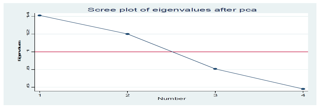
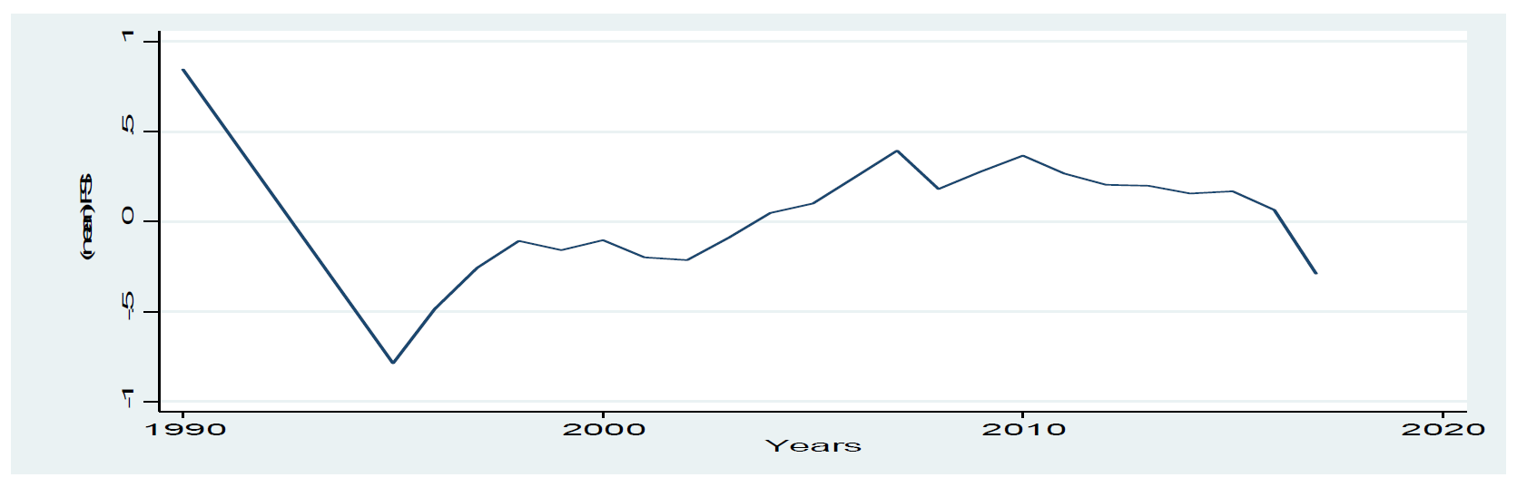
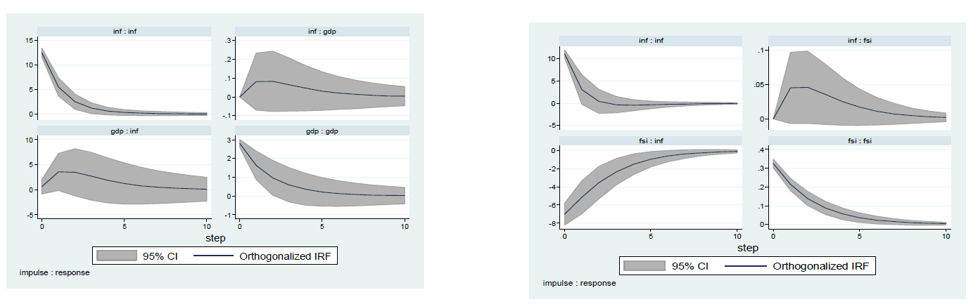
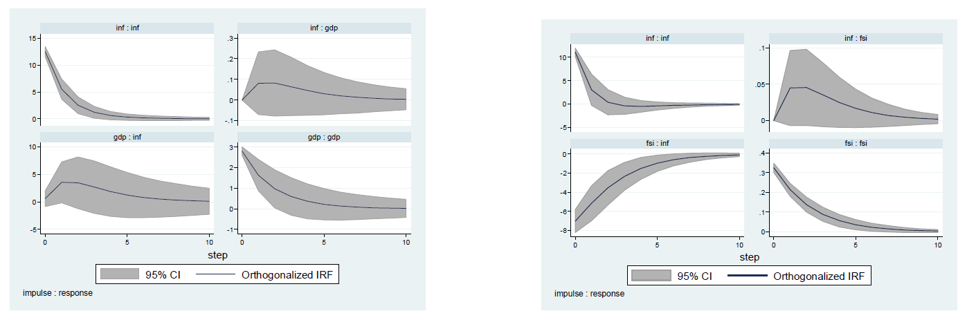
Our aim of this paper is to determine whether inflation targeting could improve economic growth and financial stability in 35 emerging economies of which 19 inflation-targeting and 16 non-inflation-targeting countries over the 1995–2017 period. To this end, we first determine the preconditions needed to adopt the inflation targeting regime using the Qualitative Comparative Analysis method (QCA). We then construct a Financial Stability Index (FSI) for emerging markets using a Principal Components Analysis (PCA). Finally, we determine the impact of shocks on economic growth and financial stability in inflation-targeting and non-inflation-targeting countries through a Panel VAR model estimated using the GMM method. The results show that some structural and institutional preconditions, should be set up during the pre-adoption period. In addition, the results indicate that the inflation-targeting regime allows emerging countries to control their economic growth and financial stability in the event of shocks to a greater extent than non-targeting countries, although the magnitude of the shock persists only in the short run, given that economic and financial conditions return to their normal state in the long run.
Citation: Ikram Ben Romdhane, Mohamed Amin Chakroun, Sami Mensi. Inflation Targeting, Economic Growth and Financial Stability: Evidence from Emerging Countries[J]. Quantitative Finance and Economics, 2023, 7(4): 697-723. doi: 10.3934/QFE.2023033
Our aim of this paper is to determine whether inflation targeting could improve economic growth and financial stability in 35 emerging economies of which 19 inflation-targeting and 16 non-inflation-targeting countries over the 1995–2017 period. To this end, we first determine the preconditions needed to adopt the inflation targeting regime using the Qualitative Comparative Analysis method (QCA). We then construct a Financial Stability Index (FSI) for emerging markets using a Principal Components Analysis (PCA). Finally, we determine the impact of shocks on economic growth and financial stability in inflation-targeting and non-inflation-targeting countries through a Panel VAR model estimated using the GMM method. The results show that some structural and institutional preconditions, should be set up during the pre-adoption period. In addition, the results indicate that the inflation-targeting regime allows emerging countries to control their economic growth and financial stability in the event of shocks to a greater extent than non-targeting countries, although the magnitude of the shock persists only in the short run, given that economic and financial conditions return to their normal state in the long run.

| [1] |
Aguilera RV, Desender KA (2012) Challenges in the measuring of comparative corporate governance: a review of the main indices. West Meets East: Building Theoretical Bridges 8: 289–322. https://doi.org/10.1108/S1479-8387(2012)0000008014 doi: 10.1108/S1479-8387(2012)0000008014

|
| [2] |
Alesina A, Summers LH (1993) Central bank independence and macroeconomics performance: some comparative evidence. J Money Credit Bank 25: 151–162. https://doi.org/10.2307/2077833 doi: 10.2307/2077833
|
| [3] |
Angeriz A, Arestis P (2007) Assessing the Performance of Inflation Targeting Lite Countries. World Econ 30: 1–25. https://doi.org/10.1111/j.1467-9701.2007.01056.x doi: 10.1111/j.1467-9701.2007.01056.x
|
| [4] |
Angeriz A, Arestis P (2008) Assessing Inflation Targeting through intervention analysis. Oxford Econ Pap 60: 293–317. https://doi.org/10.1093/oep/gpm047 doi: 10.1093/oep/gpm047
|
| [5] | Armand FA, Roger S (2013) Inflation targeting and country risk: an empirical investigation. IMF Working, Paper.No.13/21. https://doi.org/10.5089/9781475554717.001 |
| [6] | Ball L, Sheridan N (2003) Does inflation targeting matter? NBER Working Paper No.9577. Cambridge. https://doi.org/10.3386/w9577 |
| [7] | Ball L, Sheridan N (2005) Does inflation targeting matter? Chapter in Bernanke, Bens, and Michael woodford (eds), The inflation targeting debate, University of Chicago Press, 249–276. https://doi.org/10.7208/chicago/9780226044736.003.0007 |
| [8] |
Baltensperger E, Fischer AM, Jordan TJ (2007) Strong goal independence and inflation targets. Eur J Polit Econ 23: 88–105. https://doi.org/10.1016/j.ejpoleco.2006.09.014 doi: 10.1016/j.ejpoleco.2006.09.014
|
| [9] | Batini N, Laxton D (2007) Under what conditions inflation targeting can be adopted? the experience of emerging markets. Central Bank of Chile, Working Paper. No.406. |
| [10] |
Bell G, Filatotchev I, Aguilera R (2014) Corporate governance and investors perceptions of foreign ipo value: an institutional perspective. Acad Manage J 57: 301–320. https://doi.org/10.5465/amj.2011.0146 doi: 10.5465/amj.2011.0146
|
| [11] | Ben Ali MS, Krammer S (2016) The role of institutions in economic development, In: Mohamed Sami Ben Ali, Economic Development in the Middle East and North Africa, Springer, 1–25. https://doi.org/10.1057/9781137480668_1 |
| [12] | Blanchard OJ, Dell'Ariccia G, Mauro P (2010) Rethinking macroeconomic policy. IMF Staff Position. Note.No.10/03. |
| [13] | Bordo MD (2008) An historical perspective on the crisis of 2007-2008. NBER Working Paper No.14569. Available from: http://www.nber.org/papers/w14569. |
| [14] | Bordo MD, Dueker MJ, Wheelock DC (2001) Aggregate price shocks and financial instability: An historical analysis. FRB of saint louis. Working Paper 2000-005B. Available from: http://research.stlouisfed.org/wp/2000/2000-005.pdf. |
| [15] |
Bordo MD, Jeanne O (2002) Monetary policy and asset prices: does benign neglect make sense? Int Financ 5: 139–164. https://doi.org/10.1111/1468-2362.00092 doi: 10.1111/1468-2362.00092
|
| [16] |
Bordo MD, Wheelock DC (1998) Price stability and financial stability: The historical record. Rev-Fed Reserve Bank Saint Louis 80: 41–60. https://doi.org/10.20955/r.80.41-62 doi: 10.20955/r.80.41-62
|
| [17] | Borio C, English B, Filardo A (2003) A tale of two perspectives: old or new challenges for monetary policy. BIS Working Paper No.147. Available from: https://www.bis.org/publ/bppdf/bispap19a.pdf. |
| [18] | Borio C, Lowe P (2002) Asset prices, financial and monetary policy: exploring the nexus. Paper presented at the BIS Conference on "Changes in risk through time: measurement and policy options", BIS Working Papers, No.114, Basel. |
| [19] |
Borio C, Zhu H (2012) Capital regulation, risk-taking and monetary policy: A missing link in the transmission mechanism? J Financ Stab 8: 236–251. https://doi.org/10.1016/j.jfs.2011.12.003 doi: 10.1016/j.jfs.2011.12.003
|
| [20] |
Brito RD, Bystedt B (2010) Inflation targeting in emerging economies: panel evidence. J Deve Econ. 9: 198–210. https://doi.org/10.1016/j.jdeveco.2009.09.010 doi: 10.1016/j.jdeveco.2009.09.010
|
| [21] | Cecchetti S, Genberg H, Lipsky J, et al. (2000) Asset prices and central bank policy, The Geneva Report on the World Economy no. 02, International Centre for Monetary and Banking Studies, Geneva. Available from: http://down.cenet.org.cn/upfile/8/2010318204458149.pdf. |
| [22] |
Cukierman A, Webb SB, Neyapti B (1992) Measuring the independence of central bank and its effect on policy outcomes. World Bank Econ Rev. 6: 353–398. https://doi.org/10.1093/wber/6.3.353 doi: 10.1093/wber/6.3.353
|
| [23] | De Carvalho Filho MIE (2010). Inflation targeting and the crisis: An empirical assessment. International Monetary Fund. |
| [24] |
Dinabandhu S, Debashis A (2019) Monetary policy and financial stability: The rôle of inflation targeting. Aust Econ Rev 53: 50–75. https://doi.org/10.1111/1467-8462.12348 doi: 10.1111/1467-8462.12348
|
| [25] |
Dreher A, Sturm JE, De Haan J (2008) Does high inflation cause central bankers to lose their job? evidence based on a new dataset. Eur J Polit Econ 24: 778–787. https://doi.org/10.1016/j.ejpoleco.2008.04.001 doi: 10.1016/j.ejpoleco.2008.04.001
|
| [26] | Fazio DM, Silva TC, Tabak BM, et al. (2015) Inflation targeting: Is IT to blame for banking system instability. J Bank Financ 59: 76–97. http://dx.doi.org/10.1016/j.jbankfin.2015.05.016 |
| [27] |
Fazio DM, Silva TC, Tabak BM, et al. (2018) Inflation targeting and financial stability: does the quality of institutions matter? Econ Model 71: 1–15. https://doi.org/10.1016/j.econmod.2017.09.011 doi: 10.1016/j.econmod.2017.09.011
|
| [28] |
Foueijieu AA (2017) Inflation targeting and financial stability in emerging markets. Econ Model 60: 51–70. https://doi.org/10.1016/j.econmod.2016.08.020 doi: 10.1016/j.econmod.2016.08.020
|
| [29] | Foueijieu AA, Roger S (2013) Inflation targeting and country risk: an empirical investigation. IMF Working Paper No. 13/21. https://doi.org/10.5089/9781475554717.001 |
| [30] | Fouejieu AA (2014) Inflation targeters do not care (enough) about financial stability a myth?: investigation on a sample of emerging market economies. Working paper No.2013-08. |
| [31] |
Frappa S, Mésonnier JS (2010) The housing price boom of the late 1990s: did inflation targeting matter? J Financ Stab 6: 243–254. https://doi.org/10.1016/j.jfs.2010.06.001 doi: 10.1016/j.jfs.2010.06.001
|
| [32] | Ftiti Z, Essadi E (2013) Relevance of the inflation targeting policy. J Econ Financ Model. 1: 62–72. |
| [33] | Gadanecz B, Jayaram K (2008) Measures of financial stability- a review, Proceedings of the IFC conference, on "Measuring financial innovation and its impact", Basel on 26–27 august. |
| [34] | Goldfajn I, Werlang S (2000) The pass -through from depreciation to inflation: a panel study. Department of Economics Puc-Rio (Brazil). Banco Central de Brasil Working Paper No. 5. |
| [35] |
Gonçalves CES, Carvalho A (2008) Who chooses to inflation target? Econ Lett 99: 410–413. https://doi.org/10.1016/j.econlet.2007.09.022 doi: 10.1016/j.econlet.2007.09.022
|
| [36] |
Gonçalves CES, Carvalho A (2009) Inflation targeting matters: evidence from OECD economies sacrifice ratios. J Money Credit Bank 41: 233–243. https://doi.org/10.1111/j.1538-4616.2008.00195.x doi: 10.1111/j.1538-4616.2008.00195.x
|
| [37] |
Gonçalves CES, Salles JM (2008) Inflation targeting in emerging economies: what do the data Say? J Dev Econ 85: 312–318. https://doi.org/10.1016/j.jdeveco.2006.07.002 doi: 10.1016/j.jdeveco.2006.07.002
|
| [38] | Hammond G (2012) State of the art of inflation targeting: the bank of england's centre for central bank studies. CCBS Handbook.No.29. |
| [39] |
Hu Y (2006) The choice of inflation targeting: an empirical investigation. Int Econ Econ Policy 31: 27–42. https://doi.org/10.1007/s10368-005-0044-y doi: 10.1007/s10368-005-0044-y
|
| [40] |
Huang HC, Yeh CC, Wang X (2019) Inflation targeting and output-inflation tradeoffs. J Int Money Financ 96: 102–120. https://doi.org/10.1016/j.jimonfin.2019.04.009 doi: 10.1016/j.jimonfin.2019.04.009
|
| [41] | Hyvonen M (2004) Inflation convergence across countries. Reserve Bank of Australia RBA Research Sydney. Discussion Papers No.4 |
| [42] | Issing O (2003) Monetary and financial stability: is there a trade-off? Remarks at Conference on monetary stability, financial stability and the business cycle. Bank for International Settlements, Basel on 28–29, 1–7. |
| [43] |
Issing O (2009) Some Lessons from the financial market crisis. Int Financ 12: 431–444. https://doi.org/10.1111/j.1468-2362.2009.01250.x doi: 10.1111/j.1468-2362.2009.01250.x
|
| [44] |
Kadria M, Ben Aissa S (2014) Implementation of inflation targeting and budget deficit performance in emerging countries: a treatment effect evaluation. J Appl Bus Res 30: 1077–1090. https://doi.org/10.19030/jabr.v30i4.8656 doi: 10.19030/jabr.v30i4.8656
|
| [45] |
Kadria M, Ben Aissa S (2016) Inflation targeting and public deficit in emerging countries: A time varying treatment effect approach. Econ Model 52: 108–114. https://doi.org/10.1016/j.econmod.2015.02.022 doi: 10.1016/j.econmod.2015.02.022
|
| [46] | Leijonhufvud A (2007) Monetary and financial stability. CEPR Policy Insight. No.14. Available from: https://cepr.org/sites/default/files/policy_insights/PolicyInsight14.pdf. |
| [47] | Levya G (2008) The Choice of inflation targeting. Working Papers Central Bank of Chile. No.475. |
| [48] |
Lin S, Ye H (2007) Does inflation targeting really make a difference? evaluating the treatment effect of inflation targeting in seven industrial economies. J Monetary Econ 54: 2521–2533. https://doi.org/10.1016/j.jmoneco.2007.06.017 doi: 10.1016/j.jmoneco.2007.06.017
|
| [49] |
Lin S, Ye H (2009) Does inflation targeting make a difference in developing countries? J Dev Econ 89: 118–123. https://doi.org/10.1016/j.jdeveco.2008.04.006 doi: 10.1016/j.jdeveco.2008.04.006
|
| [50] |
Lin S, Ye H (2010) On the international effects of inflation targeting. Rev Econ Stat 92: 195–199. https://doi.org/10.1162/rest.2009.11553 doi: 10.1162/rest.2009.11553
|
| [51] |
Lucotte Y (2012) Adoption of inflation targeting and tax revenue performance in emerging market economies: an empirical investigation. Econ Syst 36: 609–628. https://doi.org/10.1016/j.ecosys.2012.01.001 doi: 10.1016/j.ecosys.2012.01.001
|
| [52] | Mahadeva L, Sterne G (2000) Monetary policy frameworks in a global context, Routledge, London. https://doi.org/10.4324/9780203351147 |
| [53] |
Marcel F, Cristoph GS, Malte R (2020) Inflation targeting as a shock absorber. J Int Econ 123: 103308. https://doi.org/10.1016/j.jinteco.2020.103308 doi: 10.1016/j.jinteco.2020.103308
|
| [54] |
Michael R, Abrigo M, Love I (2016) Estimation of panel vector autoregression in stata: a package of programs. Stata J 16: 778–804. https://doi.org/10.1177/1536867X1601600314 doi: 10.1177/1536867X1601600314
|
| [55] | Mishkin FS (2004) Can inflation targeting work in emerging market countries? NBER Working Paper. No. 10646. https://doi.org/10.3386/w10646 |
| [56] | Mishkin FS (2011) Monetary policy strategy: lessons from the crisis. NBER Working Paper. No.16755. https://doi.org/10.3386/w16755 |
| [57] | Mishkin FS, Schmidt-Hebbel K (2001) One decade of inflation targeting in the world: what do we know and what do we need to know? NBER Working Paper No.8397. Cambridge. https://doi.org/10.3386/w8397 |
| [58] | Mishkin FS, Schmidt-Hebbel K (2007) Does inflation targeting make a difference? In: Mishkin, Frederic, and Klaus Schimdt –Hebbel (eds), Monetary policy under inflation targeting, 11, Center Banking, Analysis, and Economic Policies, Central Bank of Chile, 291–372. https://doi.org/10.3386/w12876 |
| [59] |
Mukherjee B, Singer DA (2008) Monetary institutions, partisanship, and inflation targeting. Int Organ 62: 323–358. https://doi.org/10.1017/S0020818308080119 doi: 10.1017/S0020818308080119
|
| [60] | Munoz F, Schmidt-Hebbel K (2012) Do the world's central banks react to financial markets? Working Paper held jointly by the International Monetary Fund, the World Bank, the Consortium on Financial Systems and Poverty, and the UK Department for International Development in September. Available from: http://www.cfsp.org/publications/working-papers/do-worlds-central-banks-react-financial-markets#.X3RvXVUzbIU. |
| [61] |
Nair AR, Anand B (2020) Monetary policy and financial stability: should central bank lean against the wind? Central Bank Rev 20: 133–142. https://doi.org/10.1016/j.cbrev.2020.03.006 doi: 10.1016/j.cbrev.2020.03.006
|
| [62] |
Omid MA, Kundan NK, Kishorb S (2018) Re-evaluating the effectiveness of inflation targeting. J Econ Dyn Control 90: 76-97. https://doi.org/10.1016/j.jedc.2018.01.045 doi: 10.1016/j.jedc.2018.01.045
|
| [63] | Pétursson TG (2009) Inflation control around the world: why are some countries more successful than others? Central Bank of Iceland. Working Paper. No. 42, Department of Economics, Central Bank of Iceland. https://doi.org/10.1017/CBO9780511779770.007 |
| [64] | Pierre RA, Luiz AP, Da S (2013) Inflation targeting and financial Stability: a perspective from the developing world. Banco central do Brasil Working Paper.No.324, 1–116. |
| [65] |
Posen AS (2006) Why central banks should not burst bubbles. Int Financ 9: 109–124. https://doi.org/10.1111/j.1468-2362.2006.00028.x doi: 10.1111/j.1468-2362.2006.00028.x
|
| [66] | Ragin CC (1987) The comparative method. moving beyond qualitative and quantitative strategies, Berkeley and Los Angeles: University of California Press. |
| [67] | Rajan R (2005) Has financial development made the world riskier? In the greenspan era: lessons for the future, Proceedings of the FRB of Kansas City Economic Symposium, Jackson Hole, 313–369. https://doi.org/10.3386/w11728 |
| [68] |
Rihoux B (2006) Qualitative comparative analysis (QCA) and related systematic comparative methods: recent advances and remaining challenges for social science research. Int Sociol 21: 679–706. https://doi.org/10.1177/0268580906067836 doi: 10.1177/0268580906067836
|
| [69] |
Roubini N (2006) Why central banks should burst bubbles? Int Financ 9: 87–107. https://doi.org/10.1111/j.1468-2362.2006.00032.x doi: 10.1111/j.1468-2362.2006.00032.x
|
| [70] | Samaryna H, De Haan J (2011) Right on target: exploring the determinants of inflation targeting adoption. DNB Working Paper No.321. De Nederlandsche Bank. https://doi.org/10.2139/ssrn.1957602 |
| [71] |
Schwartz A (1995) Why financial stability depends on price stability? Econ Affairs 15: 21–25. https://doi.org/10.1111/j.1468-0270.1995.tb00493.x doi: 10.1111/j.1468-0270.1995.tb00493.x
|
| [72] |
Seow SK, Siong HL, Mansor HI (2017) Credit expansion and financial stability in malaysia. Econ Model 61: 339–350. https://doi.org/10.1016/j.econmod.2016.10.013 doi: 10.1016/j.econmod.2016.10.013
|
| [73] | Svensson LEO (2010) Inflation targeting, In: Durlauf S.N., Blume L.E. (eds), Monetary Economics. The New Palgrave Economics Collection, Palgrave Macmillan, London. |
| [74] | Taylor JB (2009) The financial crisis and the policy responses: an empirical analysis of what went wrong. NBER Working Paper. No.14631. https://doi.org/10.3386/w14631 |
| [75] | Truman EM (2003) Inflation targeting in the world economy. Peterson Institute for International Economics. Washington D.C. |
| [76] |
Umar M, Wen J (2020) Does inflation targeting cause financial instability?: an empirical test of paradox of credibility hypothesis. N Am J Econ Financ 52. https://doi.org/10.1016/j.najef.2020.101164 doi: 10.1016/j.najef.2020.101164
|
| [77] | Vega M, Winkelried D (2005) Inflation targeting and inflation behavior. Int J Central Bank 1: 153–176. |
| [78] | Vis B (2012) The comparative advantages of fsQCA and regression analysis for moderately large-N analyses. Sociol Methods Res 41: 168–198. |
| [79] |
Wagemann C, Buche J, Siewert MB (2016) QCA and business research: work in progress or a consolidated agenda? J Bus Res 69: 2531–2540. https://doi.org/10.1016/j.jbusres.2015.10.010 doi: 10.1016/j.jbusres.2015.10.010
|
| [80] | White WR (2006) Procyclicality in the financial system: do we need a new macrofinancial stabilisation framework? BIS. Working paper. No.193. |
| [81] | Woodford M (2012) Inflation targeting and financial stability. NBER Working Paper. No.17967. https://doi.org/10.3386/w17967 |
| [82] |
Yasuo H, Takushi K, Willem VZ (2020) Monetary policy and macroeconomic stability revisited. Rev Econ Dyn 37: 255–274. https://doi.org/10.1016/j.red.2020.03.001 doi: 10.1016/j.red.2020.03.001
|
 QFE-07-04-033-s001.pdf QFE-07-04-033-s001.pdf |
 |
Figures(8) / Tables(11)

Ikram Ben Romdhane, Mohamed Amin Chakroun, Sami Mensi. Inflation Targeting, Economic Growth and Financial Stability: Evidence from Emerging Countries[J]. Quantitative Finance and Economics, 2023, 7(4): 697-723. doi: 10.3934/QFE.2023033


 DownLoad: