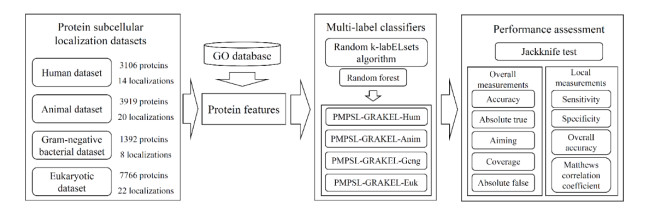
Protein functions are closely related to their subcellular locations. At present, the prediction of protein subcellular locations is one of the most important problems in protein science. The evident defects of traditional methods make it urgent to design methods with high efficiency and low costs. To date, lots of computational methods have been proposed. However, this problem is far from being completely solved. Recently, some multi-label classifiers have been proposed to identify subcellular locations of human, animal, Gram-negative bacterial and eukaryotic proteins. These classifiers adopted the protein features derived from gene ontology information. Although they provided good performance, they can be further improved by adopting more powerful machine learning algorithms. In this study, four improved multi-label classifiers were set up for identification of subcellular locations of the above four protein types. The random k-labelsets (RAKEL) algorithm was used to tackle proteins with multiple locations, and random forest was used as the basic prediction engine. All classifiers were tested by jackknife test, indicating their high performance. Comparisons with previous classifiers further confirmed the superiority of the proposed classifiers.
Citation: Lei Chen, Ruyun Qu, Xintong Liu. Improved multi-label classifiers for predicting protein subcellular localization[J]. Mathematical Biosciences and Engineering, 2024, 21(1): 214-236. doi: 10.3934/mbe.2024010
Protein functions are closely related to their subcellular locations. At present, the prediction of protein subcellular locations is one of the most important problems in protein science. The evident defects of traditional methods make it urgent to design methods with high efficiency and low costs. To date, lots of computational methods have been proposed. However, this problem is far from being completely solved. Recently, some multi-label classifiers have been proposed to identify subcellular locations of human, animal, Gram-negative bacterial and eukaryotic proteins. These classifiers adopted the protein features derived from gene ontology information. Although they provided good performance, they can be further improved by adopting more powerful machine learning algorithms. In this study, four improved multi-label classifiers were set up for identification of subcellular locations of the above four protein types. The random k-labelsets (RAKEL) algorithm was used to tackle proteins with multiple locations, and random forest was used as the basic prediction engine. All classifiers were tested by jackknife test, indicating their high performance. Comparisons with previous classifiers further confirmed the superiority of the proposed classifiers.

| [1] |
K. C. Chou, H. B. Shen, Recent progress in protein subcellular location prediction, Anal. Biochem., 370 (2007), 1–16. https://doi.org/10.1016/j.ab.2007.07.006 doi: 10.1016/j.ab.2007.07.006

|
| [2] | R. F. Murphy, M. V. Boland, M. Velliste, Towards a systematics for protein subcellular location: quantitative description of protein localization patterns and automated analysis of fluorescence microscope images, in Proceedings International Conference on Intelligent System Molecular Biology, 8 (2000), 251–259. |
| [3] |
J. Cao, W. Liu, J. He, H. Gu, Mining proteins with non-experimental annotations based on an active sample selection strategy for predicting protein subcellular localization, PLoS One, 8 (2013), e67343. https://doi.org/10.1371/journal.pone.0067343 doi: 10.1371/journal.pone.0067343
|
| [4] |
H. B. Shen, J. Yang, K. C. Chou, Methodology development for predicting subcellular localization and other attributes of proteins, Expert Rev. Proteomics, 4 (2007), 453–463. https://doi.org/10.1586/14789450.4.4.453 doi: 10.1586/14789450.4.4.453
|
| [5] |
A. Reinhardt, T. Hubbard, Using neural networks for prediction of the subcellular location of proteins, Nucleic Acids Res., 26 (1998), 2230–2236. https://doi.org/10.1093/nar/26.9.2230 doi: 10.1093/nar/26.9.2230
|
| [6] |
J. Cedano, P. Aloy, J. A. Perez-Pons, E. Querol, Relation between amino acid composition and cellular location of proteins, J. Mol. Biol., 266 (1997), 594–600. https://doi.org/10.1006/jmbi.1996.0804 doi: 10.1006/jmbi.1996.0804
|
| [7] |
Y. X. Pan, Z. Z. Zhang, Z. M. Guo, G. Y. Feng, Z. D. Huang, L. He, Application of pseudo amino acid composition for predicting protein subcellular location: stochastic signal processing approach, J. Protein Chem., 22 (2003), 395–402. https://doi.org/10.1023/a:1025350409648 doi: 10.1023/a:1025350409648
|
| [8] |
J. Y. Shi, S. Zhang, Q. Pan, G. Zhou, Using pseudo amino acid composition to predict protein subcellular location: approached with amino acid composition distribution, Amino Acids, 35 (2008), 321–327. https://doi.org/10.1007/s00726-007-0623-z doi: 10.1007/s00726-007-0623-z
|
| [9] |
H. Lin, H. Ding, F. Guo, A. Zhang, J. Huang, Predicting subcellular localization of mycobacterial proteins by using Chou's pseudo amino acid composition, Protein Pept. Lett., 15 (2008), 739–744. https://doi.org/10.2174/092986608785133681 doi: 10.2174/092986608785133681
|
| [10] |
K. Chou, Prediction of protein cellular attributes using pseudo-amino acid composition, Proteins, 43 (2001), 246–255. https://doi.org/10.1002/prot.1035 doi: 10.1002/prot.1035
|
| [11] |
T. Liu, X. Zheng, C. Wang, J. Wang, Prediction of subcellular location of apoptosis proteins using pseudo amino acid composition: an approach from auto covariance transformation, Protein Pept. Lett., 17 (2010), 1263–1269. https://doi.org/10.2174/092986610792231528 doi: 10.2174/092986610792231528
|
| [12] |
Y. Shen, J. Tang, F. Guo, Identification of protein subcellular localization via integrating evolutionary and physicochemical information into Chou's general PseAAC, J. Theor. Biol., 462 (2019), 230–239. https://doi.org/10.1016/j.jtbi.2018.11.012 doi: 10.1016/j.jtbi.2018.11.012
|
| [13] |
Y. H. Yao, Z. X. Shi, Q. Dai, Apoptosis protein subcellular location prediction based on position-specific scoring matrix, J. Comput. Theor. Nanos., 11 (2014), 2073–2078. https://doi.org/10.1166/jctn.2014.3607 doi: 10.1166/jctn.2014.3607
|
| [14] |
T. Liu, P. Tao, X. Li, Y. Qin, C. Wang, Prediction of subcellular location of apoptosis proteins combining tri-gram encoding based on PSSM and recursive feature elimination, J. Theor. Biol., 366 (2015), 8–12. https://doi.org/10.1016/j.jtbi.2014.11.010 doi: 10.1016/j.jtbi.2014.11.010
|
| [15] |
S. Wang, W. Li, Y. Fei, An improved process for generating uniform PSSMs and its application in protein subcellular localization via various global dimension reduction techniques, IEEE Access, 7 (2019), 42384–42395. https://doi.org/10.1109/ACCESS.2019.2907642 doi: 10.1109/ACCESS.2019.2907642
|
| [16] |
X. Cheng, X. Xiao, K. C. Chou, pLoc-mHum: predict subcellular localization of multi-location human proteins via general PseAAC to winnow out the crucial GO information. Bioinformatics, 34 (2018), 1448–1456. https://doi.org/10.1093/bioinformatics/btx711 doi: 10.1093/bioinformatics/btx711
|
| [17] |
X. Cheng, S. Zhao, W. Lin, X. Xiao, K. Chou, pLoc-mAnimal: predict subcellular localization of animal proteins with both single and multiple sites, Bioinformatics, 33 (2017), 3524–3531. https://doi.org/10.1093/bioinformatics/btx476 doi: 10.1093/bioinformatics/btx476
|
| [18] |
X. Cheng, X. Xiao, K.C. Chou, pLoc-mGneg: Predict subcellular localization of Gram-negative bacterial proteins by deep gene ontology learning via general PseAAC, Genomics, 110 (2017), 231–239. https://doi.org/10.1016/j.ygeno.2017.10.002 doi: 10.1016/j.ygeno.2017.10.002
|
| [19] |
X. Cheng, X. Xiao, K. C. Chou, pLoc-mEuk: Predict subcellular localization of multi-label eukaryotic proteins by extracting the key GO information into general PseAAC, Genomics, 110 (2018), 50–58. https://doi.org/10.1016/j.ygeno.2017.08.005 doi: 10.1016/j.ygeno.2017.08.005
|
| [20] |
K. Chou, Y. Cai, A new hybrid approach to predict subcellular localization of proteins by incorporating gene ontology, Biochem. Biophys. Res. Commun., 311 (2003), 743–747. https://doi.org/10.1016/j.bbrc.2003.10.062 doi: 10.1016/j.bbrc.2003.10.062
|
| [21] |
S. Wan, M. Mak, S. Kung, GOASVM: A subcellular location predictor by incorporating term-frequency gene ontology into the general form of Chou's pseudo-amino acid composition, J. Theor. Biol., 323 (2013), 40–48. https://doi.org/10.1016/j.jtbi.2013.01.012 doi: 10.1016/j.jtbi.2013.01.012
|
| [22] |
S. Wan, M. Mak, S. Kung, mGOASVM: Multi-label protein subcellular localization based on gene ontology and support vector machines, BMC Bioinf., 13 (2012), 290. https://doi.org/10.1186/1471-2105-13-290 doi: 10.1186/1471-2105-13-290
|
| [23] |
K. C. Chou, Y. D. Cai, Using functional domain composition and support vector machines for prediction of protein subcellular location, J. Biol. Chem., 277 (2002), 45765–45769. https://doi.org/10.1074/jbc.M204161200 doi: 10.1074/jbc.M204161200
|
| [24] |
K. Chou, H. Shen, A new method for predicting the subcellular localization of eukaryotic proteins with both single and multiple sites: Euk-mPLoc 2.0, PLoS One, 5 (2010), e9931. https://doi.org/10.1371/journal.pone.0009931 doi: 10.1371/journal.pone.0009931
|
| [25] |
Y. Cai, K. Chou, Nearest neighbour algorithm for predicting protein subcellular location by combining functional domain composition and pseudo-amino acid composition, Biochem. Biophys. Res. Commun., 305 (2003), 407–411. https://doi.org/10.1016/s0006-291x(03)00775-7 doi: 10.1016/s0006-291x(03)00775-7
|
| [26] |
K. Chou, Y. Cai, Predicting subcellular localization of proteins by hybridizing functional domain composition and pseudo-amino acid composition, J. Cell. Biochem., 91 (2004), 1197–1203. https://doi.org/10.1002/jcb.10790 doi: 10.1002/jcb.10790
|
| [27] |
X. Pan, L. Chen, M. Liu, Z. Niu, T. Huang, Y. Cai, Identifying protein subcellular locations with embeddings-based node2loc, IEEE/ACM Trans. Comput. Biol. Bioinf., 19 (2022), 666–675. https://doi.org/10.1109/TCBB.2021.3080386 doi: 10.1109/TCBB.2021.3080386
|
| [28] |
X. Pan, H. Li, T. Zeng, Z. Li, L. Chen, T. Huang, et al., Identification of protein subcellular localization with network and functional embeddings, Front. Genet., 11 (2021), 626500. https://doi.org/10.3389/fgene.2020.626500 doi: 10.3389/fgene.2020.626500
|
| [29] |
H. Liu, B. Hu, L. Chen, Identifying protein subcellular location with embedding features learned from networks, Curr. Proteomics, 18 (2021), 646–660. https://doi.org/10.2174/1570164617999201124142950 doi: 10.2174/1570164617999201124142950
|
| [30] | R. Wang, L. Chen, Identification of human protein subcellular location with multiple networks, Curr. Proteomics, 19 (2022), 344–356. |
| [31] |
R. Su, L. He, T. Liu, X. Liu, L. Wei, Protein subcellular localization based on deep image features and criterion learning strategy, Briefings Bioinf., 22 (2020), bbaa313. https://doi.org/10.1093/bib/bbaa313 doi: 10.1093/bib/bbaa313
|
| [32] |
M. Ullah, F. Hadi, J. Song, D. Yu, PScL-DDCFPred: an ensemble deep learning-based approach for characterizing multiclass subcellular localization of human proteins from bioimage data, Bioinformatics, 38 (2022), 4019–4026. https://doi.org/10.1093/bioinformatics/btac432 doi: 10.1093/bioinformatics/btac432
|
| [33] |
M. Ullah, K. Han, F. Hadi, J. Xu, J. Song, D. Yu, PScL-HDeep: image-based prediction of protein subcellular location in human tissue using ensemble learning of handcrafted and deep learned features with two-layer feature selection, Briefings Bioinf., 22 (2021), bbab278. https://doi.org/10.1093/bib/bbab278 doi: 10.1093/bib/bbab278
|
| [34] | G. Tsoumakas, I. Vlahavas, Random k-Labelsets: An ensemble method for multilabel classification, in Machine Learning: ECML 2007, (2007), 406–417. https://doi.org/10.1007/978-3-540-74958-5_38 |
| [35] |
L. Breiman, Random forests, Mach. Learn., 45 (2001), 5–32. https://doi.org/10.1023/A:1010933404324 doi: 10.1023/A:1010933404324
|
| [36] |
K. C. Chou, Z. C. Wu, X. Xiao, iLoc-Hum: using the accumulation-label scale to predict subcellular locations of human proteins with both single and multiple sites, Mol. Biosyst., 8 (2012), 629–641. https://doi.org/10.1039/c1mb05420a doi: 10.1039/c1mb05420a
|
| [37] |
H. B. Shen, K. C. Chou, A top-down approach to enhance the power of predicting human protein subcellular localization: Hum-mPLoc 2.0, Anal. Biochem., 394 (2009), 269–274. https://doi.org/10.1016/j.ab.2009.07.046 doi: 10.1016/j.ab.2009.07.046
|
| [38] |
W. Z. Lin, J. Fang, X. Xiao, K. Chou, iLoc-Animal: a multi-label learning classifier for predicting subcellular localization of animal proteins, Mol. Biosyst., 9 (2013), 634–644. https://doi.org/10.1039/c3mb25466f doi: 10.1039/c3mb25466f
|
| [39] |
H. B. Shen, K. C. Chou, Gneg-mPLoc: a top-down strategy to enhance the quality of predicting subcellular localization of Gram-negative bacterial proteins, J. Theor. Biol., 264 (2010), 326–333. https://doi.org/10.1016/j.jtbi.2010.01.018 doi: 10.1016/j.jtbi.2010.01.018
|
| [40] |
X. Xiao, Z. C. Wu, K. C. Chou, A multi-label classifier for predicting the subcellular localization of gram-negative bacterial proteins with both single and multiple sites, PLoS One, 6 (2011), e20592. https://doi.org/10.1371/journal.pone.0020592 doi: 10.1371/journal.pone.0020592
|
| [41] |
G. Tsoumakas, I. Katakis, Multi-label classification: An overview, Int. J. Data Warehouse. Min., 3 (2007), 1–13. https://doi.org/10.4018/jdwm.2007070101 doi: 10.4018/jdwm.2007070101
|
| [42] | S. Al-Maadeed, Kernel collaborative label power set system for multi-label classification, in Qatar Foundation Annual Research Forum Volume 2013 Issue 1, Hamad bin Khalifa University Press, 2013 (2013). https://doi.org/10.5339/qfarf.2013.ICTP-028 |
| [43] |
J. P. Zhou, L. Chen, Z. H. Guo, iATC-NRAKEL: An efficient multi-label classifier for recognizing anatomical therapeutic chemical classes of drugs, Bioinformatics, 36 (2020), 1391–1396. https://doi.org/10.1093/bioinformatics/btz757 doi: 10.1093/bioinformatics/btz757
|
| [44] |
J. P. Zhou, L. Chen, T. Wang, M. Liu, iATC-FRAKEL: A simple multi-label web-server for recognizing anatomical therapeutic chemical classes of drugs with their fingerprints only, Bioinformatics, 36 (2020), 3568–3569. https://doi.org/10.1093/bioinformatics/btaa166 doi: 10.1093/bioinformatics/btaa166
|
| [45] |
X. Li, L. Lu, L. Chen, Identification of protein functions in mouse with a label space partition method, Math. Biosci. Eng., 19 (2022), 3820–3842. https://doi.org/10.3934/mbe.2022176 doi: 10.3934/mbe.2022176
|
| [46] |
H. Li, S. Zhang, L. Chen, X. Pan, Z. Li, T. Huang, et al., Identifying functions of proteins in mice with functional embedding features, Front. Genet., 13 (2022), 909040. https://doi.org/10.3389/fgene.2022.909040 doi: 10.3389/fgene.2022.909040
|
| [47] |
L. Chen, Z. Li, T. Zeng, Y. Zhang, H. Li, T. Huang, et al., Predicting gene phenotype by multi-label multi-class model based on essential functional features, Mol. Genet. Genomics, 296 (2021), 905–918. https://doi.org/10.1007/s00438-021-01789-8 doi: 10.1007/s00438-021-01789-8
|
| [48] |
Y. Zhu, B. Hu, L. Chen, Q. Dai, iMPTCE-Hnetwork: a multi-label classifier for identifying metabolic pathway types of chemicals and enzymes with a heterogeneous network, Comput. Math. Methods Med., 2021 (2021), 6683051. https://doi.org/10.1155/2021/6683051 doi: 10.1155/2021/6683051
|
| [49] |
J. Che, L. Chen, Z. Guo, S. Wang, Aorigele, Drug target group prediction with multiple drug networks, Comb. Chem. High Throughput Screen., 23 (2020), 274–284. https://doi.org/10.2174/1386207322666190702103927 doi: 10.2174/1386207322666190702103927
|
| [50] |
H. Wang, L. Chen, PMPTCE-HNEA: Predicting metabolic pathway types of chemicals and enzymes with a heterogeneous network embedding algorithm, Curr. Bioinf., 18 (2023), 748–759. https://doi.org/10.2174/1574893618666230224121633 doi: 10.2174/1574893618666230224121633
|
| [51] | J. Read, P. Reutemann, B. Pfahringer, MEKA: A multi-label/multi-target extension to WEKA, J. Mach. Learn. Res., 17 (2016), 1–5. |
| [52] |
B. Ran, L. Chen, M. Li, Y. Han, Q. Dai, Drug-Drug interactions prediction using fingerprint only, Comput. Math. Methods Med., 2022 (2022), 7818480. https://doi.org/10.1155/2022/7818480 doi: 10.1155/2022/7818480
|
| [53] |
M. Onesime, Z. Yang, Q. Dai, Genomic island prediction via chi-square test and random forest algorithm, Comput. Math. Methods Med., 2021 (2021), 9969751. https://doi.org/10.1155/2021/9969751 doi: 10.1155/2021/9969751
|
| [54] |
L. Chen, K. Chen, B. Zhou, Inferring drug-disease associations by a deep analysis on drug and disease networks, Math. Biosci. Eng., 20 (2023), 14136–14157. https://doi.org/10.3934/mbe.2023632 doi: 10.3934/mbe.2023632
|
| [55] |
P. Chen, T. Shen, Y. Zhang, B. Wang, A sequence-segment neighbor encoding schema for protein hotspot residue prediction, Curr. Bioinf., 15 (2020), 445–454. https://doi.org/10.2174/1574893615666200106115421 doi: 10.2174/1574893615666200106115421
|
| [56] |
Z. B. Lv, J. Zhang, H. Ding, Q. Zou, RF-PseU: A random forest predictor for rna pseudouridine sites, Front. Bioeng. Biotechnol., 8 (2020), 134. https://doi.org/10.3389/fbioe.2020.00134 doi: 10.3389/fbioe.2020.00134
|
| [57] |
F. Huang, Q. Ma, J. Ren, J. Li, F. Wang, T. Huang, et al., Identification of smoking associated transcriptome aberration in blood with machine learning methods, Biomed. Res. Int., 2023 (2023), 445–454. https://doi.org/10.1155/2023/5333361 doi: 10.1155/2023/5333361
|
| [58] |
F. Huang, M. Fu, J. Li, L. Chen, K. Feng, T. Huang, et al., Analysis and prediction of protein stability based on interaction network, gene ontology, and kegg pathway enrichment scores, Biochim. Biophys. Acta. Proteins Proteom., 1871 (2023), 140889. https://doi.org/10.1016/j.bbapap.2023.140889 doi: 10.1016/j.bbapap.2023.140889
|
| [59] |
J. Ren, Y. Zhang, W. Guo, K. Feng, Y. Yuan, T. Huang, et al., Identification of genes associated with the impairment of olfactory and gustatory functions in COVID-19 via machine-learning methods, Life (Basel), 13 (2023), 798. https://doi.org/10.3390/life13030798 doi: 10.3390/life13030798
|
| [60] |
K. C. Chou, C. T. Zhang, Prediction of protein structural classes, Crit. Rev. Biochem. Mol. Biol., 30 (1995), 275–349. https://doi.org/10.3109/10409239509083488 doi: 10.3109/10409239509083488
|
| [61] |
K. C. Chou, Z. C. Wu, X. Xiao, iLoc-Euk: A multi-label classifier for predicting the subcellular localization of singleplex and multiplex eukaryotic proteins, PLoS One, 6 (2011), e18258. https://doi.org/10.1371/journal.pone.0018258 doi: 10.1371/journal.pone.0018258
|
| [62] | S. Tang, L. Chen, iATC-NFMLP: Identifying classes of anatomical therapeutic chemicals based on drug networks, fingerprints and multilayer perceptron. Curr. Bioinf., 17 (2022), 814–824. |
| [63] |
H. Zhao, Y. Li, J. Wang, A convolutional neural network and graph convolutional network-based method for predicting the classification of anatomical therapeutic chemicals, Bioinformatics, 37 (2021), 2841–2847. https://doi.org/10.1093/bioinformatics/btab204 doi: 10.1093/bioinformatics/btab204
|
| [64] |
W. Chen, H. Yang, P. Feng, H. Ding, H. Lin, iDNA4mC: identifying DNA N4-methylcytosine sites based on nucleotide chemical properties, Bioinformatics, 33 (2017), 3518–3523. https://doi.org/10.1093/bioinformatics/btx479 doi: 10.1093/bioinformatics/btx479
|
| [65] |
L. Wei, P. Xing, R. Su, G. Shi, Z. S. Ma, Q. Zou, CPPred-RF: A sequence-based predictor for identifying cell-penetrating peptides and their uptake efficiency, J. Proteome Res., 16 (2017), 2044–2053. https://doi.org/10.1021/acs.jproteome.7b00019 doi: 10.1021/acs.jproteome.7b00019
|
| [66] |
S. R. Safavian, D. Landgrebe, A survey of decision tree classifier methodology, T-SMCA, 21 (1991), 660–674. https://doi.org/10.1109/21.97458 doi: 10.1109/21.97458
|
| [67] |
C. Cortes, V. Vapnik, Support-vector networks, Mach. Learn., 20 (1995), 273–297. https://doi.org/10.1007/BF00994018 doi: 10.1007/BF00994018
|
 mbe-21-01-010-supplementary.pdf mbe-21-01-010-supplementary.pdf |
 |
Figures(10) / Tables(4)

Lei Chen, Ruyun Qu, Xintong Liu. Improved multi-label classifiers for predicting protein subcellular localization[J]. Mathematical Biosciences and Engineering, 2024, 21(1): 214-236. doi: 10.3934/mbe.2024010


 DownLoad: