Oncology research has focused extensively on estrogen hormones and their function in breast cancer proliferation. Mathematical modeling is essential for the analysis and simulation of breast cancers. This research presents a novel approach to examine the therapeutic and inhibitory effects of hormone and estrogen therapies on the onset of breast cancer. Our proposed mathematical model comprises a nonlinear coupled system of partial differential equations, capturing intricate interactions among estrogen, cytotoxic T lymphocytes, dormant cancer cells, and active cancer cells. The model's parameters are meticulously estimated through experimental studies, and we conduct a comprehensive global sensitivity analysis to assess the uncertainty of these parameter values. Remarkably, our findings underscore the pivotal role of hormone therapy in curtailing breast tumor growth by blocking estrogen's influence on cancer cells. Beyond this crucial insight, our proposed model offers an integrated framework to delve into the complexity of tumor progression and immune response under hormone therapy. We employ diverse experimental datasets encompassing gene expression profiles, spatial tumor morphology, and cellular interactions. Integrating multidimensional experimental data with mathematical models enhances our understanding of breast cancer dynamics and paves the way for personalized treatment strategies. Our study advances our comprehension of estrogen receptor-positive breast cancer and exemplifies a transformative approach that merges experimental data with cutting-edge mathematical modeling. This framework promises to illuminate the complexities of cancer progression and therapy, with broad implications for oncology.
Citation: Abeer S. Alnahdi, Muhammad Idrees. Nonlinear dynamics of estrogen receptor-positive breast cancer integrating experimental data: A novel spatial modeling approach[J]. Mathematical Biosciences and Engineering, 2023, 20(12): 21163-21185. doi: 10.3934/mbe.2023936
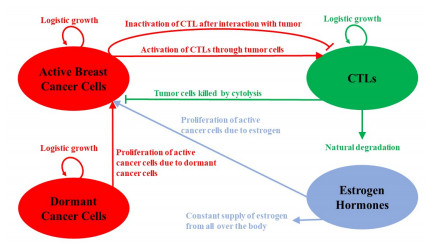
Oncology research has focused extensively on estrogen hormones and their function in breast cancer proliferation. Mathematical modeling is essential for the analysis and simulation of breast cancers. This research presents a novel approach to examine the therapeutic and inhibitory effects of hormone and estrogen therapies on the onset of breast cancer. Our proposed mathematical model comprises a nonlinear coupled system of partial differential equations, capturing intricate interactions among estrogen, cytotoxic T lymphocytes, dormant cancer cells, and active cancer cells. The model's parameters are meticulously estimated through experimental studies, and we conduct a comprehensive global sensitivity analysis to assess the uncertainty of these parameter values. Remarkably, our findings underscore the pivotal role of hormone therapy in curtailing breast tumor growth by blocking estrogen's influence on cancer cells. Beyond this crucial insight, our proposed model offers an integrated framework to delve into the complexity of tumor progression and immune response under hormone therapy. We employ diverse experimental datasets encompassing gene expression profiles, spatial tumor morphology, and cellular interactions. Integrating multidimensional experimental data with mathematical models enhances our understanding of breast cancer dynamics and paves the way for personalized treatment strategies. Our study advances our comprehension of estrogen receptor-positive breast cancer and exemplifies a transformative approach that merges experimental data with cutting-edge mathematical modeling. This framework promises to illuminate the complexities of cancer progression and therapy, with broad implications for oncology.

| [1] |
M. Arnold, E. Morgan, H. Rumgay, A. Mafra, D. Singh, M. Laversanne, et al., Current and future burden of breast cancer: Global statistics for 2020 and 2040, Breast, 66 (2022), 15–23. https://doi.org/10.1016/j.breast.2022.08.010 doi: 10.1016/j.breast.2022.08.010

|
| [2] | G. N. Sharma, R. Dave, J. Sanadya, P. Sharma, K. Sharma, Various types and management of breast cancer: An overview, J. Adv. Pharm. Technol. Res., 1 (2010), 109. |
| [3] |
Y. Feng, M. Spezia, S. Huang, C. Yuan, Z. Zeng, L. Zhang, et al., Breast cancer development and progression: Risk factors, cancer stem cells, signaling pathways, genomics, and molecular pathogenesis, Genes Dis., 5 (2018), 77–106. https://doi.org/10.1016/j.gendis.2018.05.001 doi: 10.1016/j.gendis.2018.05.001
|
| [4] |
C. Urbaniak, G. B. Gloor, M. Brackstone, L. Scott, M. Tangney, G. Reid, The microbiota of breast tissue and its association with breast cancer, Appl. Environ. Microbiol., 82 (2016), 5039–5048. https://doi.org/10.1128/AEM.01235-16 doi: 10.1128/AEM.01235-16
|
| [5] |
D. L. Monticciolo, M. S. Newell, L. Moy, B. Niell, B. Monsees, E. A. Sickles, Breast cancer screening in women at higher-than-average risk: Recommendations from the acr, J. Am. College Radiol., 15 (2018), 408–414. https://doi.org/10.1016/j.jacr.2017.11.034 doi: 10.1016/j.jacr.2017.11.034
|
| [6] |
B. H. Lerner, The breast cancer wars: Hope, fear, and the pursuit of a cure in twentieth-century America, Bull. His. Med., 76 (2002), 179–180. https://doi.org/10.1353/bhm.2002.0039 doi: 10.1353/bhm.2002.0039
|
| [7] |
L. Wiechmann, H. M. Kuerer, The molecular journey from ductal carcinoma in situ to invasive breast cancer, Cancer, 112 (2008), 2130–2142. https://doi.org/10.1002/cncr.23430 doi: 10.1002/cncr.23430
|
| [8] |
R. Benacka, D. Szaboova, Z. Gulasova, Z. Hertelyova, J. Radonak, Classic and new markers in diagnostics and classification of breast cancer, Cancers, 14 (2022), 5444. https://doi.org/10.3390/cancers14215444 doi: 10.3390/cancers14215444
|
| [9] | R. Sumbaly, N. Vishnusri, S. Jeyalatha, Diagnosis of breast cancer using decision tree data mining technique, Int. J. Comput. Appl., 98 (2014). https://doi.org/10.5120/17219-7456 |
| [10] |
B. Lim, W. A. Woodward, X. Wang, J. M. Reuben, N. T. Ueno, Inflammatory breast cancer biology: The tumour microenvironment is key, Nat. Rev. Cancer, 18 (2018), 485–499. ttps://doi.org/10.1038/s41568-018-0010-y doi: 10.1038/s41568-018-0010-y
|
| [11] |
M. Idrees, A. Sohail, Bio-algorithms for the modeling and simulation of cancer cells and the immune response, Bio-Algorithms Med-Syst., 17 (2021), 55–63. https://doi.org/10.1515/bams-2020-0054 doi: 10.1515/bams-2020-0054
|
| [12] | A. K. Abbas, A. H. Lichtman, S. Pillai, Basic Immunology E-Book: Functions And Disorders of The Ommune System, Elsevier Health Sciences, 2019. |
| [13] | Obstacles in the development of therapeutic cancer vaccines, Vaccines Cancer Immunother., (2019), 153–160. https://doi.org/10.1016/B978-0-12-814039-0.00012-6 |
| [14] |
R. A. Hess, D. Bunick, K. H. Lee, J. Bahr, J. A. Taylor, K. S. Korach, et al., A role for oestrogens in the male reproductive system, Nature, 390 (1997), 509–512. https://doi.org/10.1038/37352 doi: 10.1038/37352
|
| [15] |
P. Bhardwaj, C. C. Au, A. Benito-Martin, H. Ladumor, S. Oshchepkova, R. Moges, et al., Estrogens and breast cancer: Mechanisms involved in obesityrelated development, growth and progression, J. Steroid Biochem. Mol. Biol., 189 (2019), 161–170. https://doi.org/10.1016/j.jsbmb.2019.03.002 doi: 10.1016/j.jsbmb.2019.03.002
|
| [16] |
S. S. Skandalis, N. Afratis, G. Smirlaki, D. Nikitovic, A. D. Theocharis, G. N. Tzanakakis, Cross-talk between estradiol receptor and egfr/igfir signaling pathways in estrogen-responsive breast cancers: Focus on the role and impact of proteoglycans, Matrix Biol., 35 (2014), 182–193. https://doi.org/10.1016/j.matbio.2013.09.002 doi: 10.1016/j.matbio.2013.09.002
|
| [17] |
R. X. Song, Z. Zhang, R. J. Santen, Estrogen rapid action via protein complex formation involving ER$\alpha$ and Src, Trends Endocrinol. Metab., 16 (2005), 347–353. https://doi.org/10.1016/j.tem.2005.06.010 doi: 10.1016/j.tem.2005.06.010
|
| [18] |
L. Anderson, S. Jang, J. L. Yu, Qualitative behavior of systems of tumor–cd4+–cytokine interactions with treatments, Math. Methods Appl. Sci., 38 (2015), 4330–4344. https://doi.org/10.1002/mma.3370 doi: 10.1002/mma.3370
|
| [19] |
G. Song, T. Tian, X. Zhang, A mathematical model of cell-mediated immune response to tumor, Math. Biosci. Eng., 18 (2021), 373–385. https://doi.org/10.3934/mbe.2021020 doi: 10.3934/mbe.2021020
|
| [20] |
K. J. Mahasa, R. Ouifki, A. Eladdadi, L. de Pillis, A combination therapy of oncolytic viruses and chimeric antigen receptor t cells: A mathematical model proof of concept, Math. Biosci. Eng., 19 (2022), 4429–4457. https://doi.org/10.3934/mbe.2022205 doi: 10.3934/mbe.2022205
|
| [21] |
K. M. Storey, S. E. Lawler, T. L. Jackson, Modeling oncolytic viral therapy, immune checkpoint inhibition, and the complex dynamics of innate and adaptive immunity in glioblastoma treatment, Front. Physiol., 11 (2020), 151. https://doi.org/10.3389/fphys.2020.00151 doi: 10.3389/fphys.2020.00151
|
| [22] |
A. M. Jarrett, M. J. Bloom, W. Godfrey, A. K. Syed, D. A. Ekrut, L. I. Ehrlich, et al., Mathematical modelling of trastuzumabinduced immune response in an in vivo murine model of her2+ breast cancer, Math. Med. Biol., 36 (2019), 381–410. https://doi.org/10.1093/imammb/dqy014 doi: 10.1093/imammb/dqy014
|
| [23] |
H. C. Wei, Mathematical modeling of tumor growth: The MCF-7 breast cancer cell line, Math. Biosci. Eng., 16 (2019), 6512–6535. https://doi.org/10.3934/mbe.2019325 doi: 10.3934/mbe.2019325
|
| [24] |
H. C. Wei, Mathematical modeling of er-positive breast cancer treatment with azd9496 and palbociclib, AIMS Math., 5 (2020), 3446–3455. https://doi.org/10.3934/math.2020223 doi: 10.3934/math.2020223
|
| [25] |
M. T. McKenna, J. A. Weis, S. L. Barnes, D. R. Tyson, M. I. Miga, V. Quaranta, et al., A predictive mathematical modeling approach for the study of doxorubicin treatment in triple negative breast cancer, Sci. Rep., 7 (2017), 5725. https://doi.org/10.1038/s41598-017-05902-z doi: 10.1038/s41598-017-05902-z
|
| [26] |
S. I. Oke, M. B. Matadi, S. S. Xulu, Optimal control analysis of a mathematical model for breast cancer, Math. Comput. Appl., 23 (2018), 21. https://doi.org/10.3390/mca23020021 doi: 10.3390/mca23020021
|
| [27] | C. Mufudza, W. Sorofa, E. T. Chiyaka, Assessing the effects of estrogen on the dynamics of breast cancer, Comput. Math. Methods Med., 2012 (2012). https://doi.org/10.1155/2012/473572 |
| [28] |
R. Ouifki, S. I. Oke, Mathematical model for the estrogen paradox in breast cancer treatment, J. Math. Biol., 84 (2022), 28. https://doi.org/10.1007/s00285-022-01729-z doi: 10.1007/s00285-022-01729-z
|
| [29] | M. Riaz, M. T. M. van Jaarsveld, A. Hollestelle, W. J. C. Prager-van der Smissen, A. A. J. Heine, A. W. M. Boersma, et al., Mirna expression profiling of 51 human breast cancer cell lines reveals subtype and driver mutation-specific mirnas, Breast Cancer Res., 15 (2013), 33–49. https://doi.org/10.1186/bcr3415 |
| [30] |
V. A. Kuznetsov, I. A. Makalkin, M. A. Taylor, A. S. Perelson, Nonlinear dynamics of immunogenic tumors: Parameter estimation and global bifurcation analysis, Bull. Math. Biol., 56 (1994), 295–321. https://doi.org/10.1016/S0092-8240(05)80260-5 doi: 10.1016/S0092-8240(05)80260-5
|
| [31] |
S. E. Wardell, A. P. Yllanes, C. A. Chao, Y. Bae, K. J. Andreano, T. K. Desautels, et al., Pharmacokinetic and pharmacodynamic analysis of fulvestrant in preclinical models of breast cancer to assess the importance of its estrogen receptor-$\alpha$ degrader activity in antitumor efficacy, Breast Cancer Res. Treatment, 179 (2020), 67–77. https://doi.org/10.1007/s10549-019-05454-y doi: 10.1007/s10549-019-05454-y
|
| [32] |
M. R. Muller, F. Grunebach, A. Nencioni, P. Brossart, Transfection of dendritic cells with rna induces CD4-and CD8-mediated t cell immunity against breast carcinomas and reveals the immunodominance of presented t cell epitopes, J. Immunol., 170 (2003), 5892–5896. https://doi.org/10.4049/jimmunol.170.12.5892 doi: 10.4049/jimmunol.170.12.5892
|
| [33] | I. Gruber, N. Landenberger, A. Staebler, M. Hahn, D. Wallwiener, T. Fehm, Relationship between circulating tumor cells and peripheral T-cells in patients with primary breast cancer, Anticancer Res., 33 (2013), 2233–2238. |
| [34] | G. D. Smith, G. D. Smith, Numerical solution of partial differential equations: Finite difference methods, Oxford university press, 1985. |
| [35] | F. Wang, E. Hou, A direct meshless method for solving two-dimensional secondorder hyperbolic telegraph equations, J. Math., 2020 (2020). https://doi.org/10.1155/2020/8832197 |
| [36] |
F. Wang, E. Hou, S. A. Salama, M. M. A. Khater, Numerical investigation of the nonlinear fractional ostrovsky equation, Fractals, 30 (2022), 2240142. https://doi.org/10.1142/S0218348X22401429 doi: 10.1142/S0218348X22401429
|
| [37] |
K. G. Link, M. T. Stobb, J. D. Paola, K. B. Neeves, A. L. Fogelson, S. S. Sindi, et al., A local and global sensitivity analysis of a mathematical model of coagulation and platelet deposition under flow, PLoS One, 13(2018), e0200917. https://doi.org/10.1371/journal.pone.0200917 doi: 10.1371/journal.pone.0200917
|
| [38] | J. Folkman, R. Kalluri, Cancer without disease, Nature, 427 (2004), 787–787. https://doi.org/10.1038/427787a |
| [39] |
T. Fehm, V. Mueller, R. Marches, G. Klein, B. Gueckel, H. Neubauer, et al., Tumor cell dormancy: Implications for the biology and treatment of breast cancer, Apmis, 116 (2008), 742–753. https://doi.org/10.1111/j.1600-0463.2008.01047.x doi: 10.1111/j.1600-0463.2008.01047.x
|
| [40] |
O. E. Franco, A. K. Shaw, D. W. Strand, S. W. Hayward, Cancer associated fibroblasts in cancer pathogenesis, Semin. Cell Dev. Biol., 21 (2010), 33–39. https://doi.org/10.1016/j.semcdb.2009.10.010 doi: 10.1016/j.semcdb.2009.10.010
|
| [41] |
M. W. Retsky, R. Demicheli, W. J. M. Hrushesky, M. Baum, I. D. Gukas, Dormancy and surgery-driven escape from dormancy help explain some clinical features of breast cancer, Apmis, 116 (2008), 730–741. https://doi.org/10.1111/j.1600-0463.2008.00990.x doi: 10.1111/j.1600-0463.2008.00990.x
|
| [42] | M. Fernandez, M. Zhou, L. Soto-Ortiz, A computational assessment of the robustness of cancer treatments with respect to immune response strength, tumor size and resistance, Int. J. Tumor Ther., 7 (2018), 1–26. |
| [43] |
V. Valayannopoulos, F. Bajolle, J. B. Arnoux, S. Dubois, N. Sannier, C. Baussan, et al., Successful treatment of severe cardiomyopathy in glycogen storage disease type III With D, L-3-hydroxybutyrate, ketogenic and high-protein diet, Pediatr. Res., 70 (2011), 638–641. https://doi.org/10.1203/PDR.0b013e318232154f doi: 10.1203/PDR.0b013e318232154f
|
| [44] |
A. Friedman, K. L. Liao, The role of the cytokines IL-27 and IL-35 in cancer, Math. Biosci. Eng., 12 (2015), 1203. https://doi.org/10.3934/mbe.2015.12.1203 doi: 10.3934/mbe.2015.12.1203
|


Figures(8) / Tables(1)

Abeer S. Alnahdi, Muhammad Idrees. Nonlinear dynamics of estrogen receptor-positive breast cancer integrating experimental data: A novel spatial modeling approach[J]. Mathematical Biosciences and Engineering, 2023, 20(12): 21163-21185. doi: 10.3934/mbe.2023936


 DownLoad: