A common assumption is that pathogens more readily destabilize their host populations, leading to an elevated risk of driving both the host and pathogen to extinction. This logic underlies many strategies in conservation biology and pest and disease management. Yet, the interplay between pathogens and population stability likely varies across contexts, depending on the environment and traits of both the hosts and pathogens. This context-dependence may be particularly important in natural consumer-host populations where size- and stage-structured competition for resources strongly modulates population stability. Few studies, however, have examined how the interplay between size and stage structure and infectious disease shapes the stability of host populations. Here, we extend previously developed size-dependent theory for consumer-resource interactions to examine how pathogens influence the stability of host populations across a range of contexts. Specifically, we integrate a size- and stage-structured consumer-resource model and a standard epidemiological model of a directly transmitted pathogen. The model reveals surprisingly rich dynamics, including sustained oscillations, multiple steady states, biomass overcompensation, and hydra effects. Moreover, these results highlight how the stage structure and density of host populations interact to either enhance or constrain disease outbreaks. Our results suggest that accounting for these cross-scale and bidirectional feedbacks can provide key insight into the structuring role of pathogens in natural ecosystems while also improving our ability to understand how interventions targeting one may impact the other.
Citation: Jessica L. Hite, André M. de Roos. Pathogens stabilize or destabilize depending on host stage structure[J]. Mathematical Biosciences and Engineering, 2023, 20(12): 20378-20404. doi: 10.3934/mbe.2023901
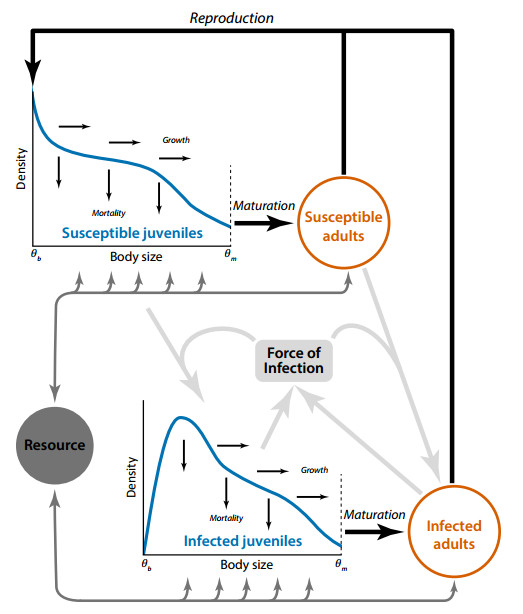
A common assumption is that pathogens more readily destabilize their host populations, leading to an elevated risk of driving both the host and pathogen to extinction. This logic underlies many strategies in conservation biology and pest and disease management. Yet, the interplay between pathogens and population stability likely varies across contexts, depending on the environment and traits of both the hosts and pathogens. This context-dependence may be particularly important in natural consumer-host populations where size- and stage-structured competition for resources strongly modulates population stability. Few studies, however, have examined how the interplay between size and stage structure and infectious disease shapes the stability of host populations. Here, we extend previously developed size-dependent theory for consumer-resource interactions to examine how pathogens influence the stability of host populations across a range of contexts. Specifically, we integrate a size- and stage-structured consumer-resource model and a standard epidemiological model of a directly transmitted pathogen. The model reveals surprisingly rich dynamics, including sustained oscillations, multiple steady states, biomass overcompensation, and hydra effects. Moreover, these results highlight how the stage structure and density of host populations interact to either enhance or constrain disease outbreaks. Our results suggest that accounting for these cross-scale and bidirectional feedbacks can provide key insight into the structuring role of pathogens in natural ecosystems while also improving our ability to understand how interventions targeting one may impact the other.

| [1] |
H. McCallum, A. Dobson, Detecting disease and parasite threats to endangered species and ecosystems, Trends Ecol. Evolut., 10 (1995), 190–194. https://doi.org/10.1016/S0169-5347(00)89050-3 doi: 10.1016/S0169-5347(00)89050-3

|
| [2] |
B. R. Forester, E. A. Beever, C. Darst, J. Szymanski, W. C. Funk, Linking evolutionary potential to extinction risk: applications and future directions, Front. Ecol. Environ., 20 (2022), 507–515. https://doi.org/10.1002/fee.2552 doi: 10.1002/fee.2552
|
| [3] | J. Bosch, A. M.-C. de Alba, S. Marquínez, S. J. Price, B. Thumsová, J. Bielby, Long-term monitoring of amphibian populations of a National Park in northern Spain reveals negative persisting effects of Ranavirus, but not Batrachochytrium dendrobatidis, Front. Veter. sci., 8 (2021). https://doi.org/10.3389/fvets.2021.645491 |
| [4] |
M. C. Fisher, T. W. Garner, Chytrid fungi and global amphibian declines, Nat. Rev. Microbiol., 18 (2020), 332–343. https://doi.org/10.1038/s41579-020-0335-x doi: 10.1038/s41579-020-0335-x
|
| [5] |
C. X. Cunningham, S. Comte, H. McCallum, D. G. Hamilton, R. Hamede, A. Storfer, et al., Quantifying 25 years of disease-caused declines in Tasmanian devil populations: host density drives spatial pathogen spread, Ecol. Letters, 24 (2021), 958–969. https://doi.org/10.1111/ele.13703 doi: 10.1111/ele.13703
|
| [6] |
D. F. Jacobs, H. J. Dalgleish, C. D. Nelson, A conceptual framework for restoration of threatened plants: The effective model of American chestnut (Castanea dentata) reintroduction, New Phytolog., 197 (2013), 378–393. https://doi.org/10.1111/nph.12020 doi: 10.1111/nph.12020
|
| [7] |
F. De Castro, B. Bolker. Mechanisms of disease-induced extinction, Ecol. Letters, 8 (2005), 117–126. https://doi.org/10.1111/j.1461-0248.2004.00693.x doi: 10.1111/j.1461-0248.2004.00693.x
|
| [8] | J. L. Hite, J. Bosch, S. Fernández-Beaskoetxea, D. Medina, S. R. Hall, Joint effects of habitat, zooplankton, host stage structure and diversity on amphibian chytrid, Proceed. Royal Soc. B Biol. Sci., 283 (2016), 20160832. https://doi.org/10.1098/rspb.2016.0832 |
| [9] | C. G. Becker, S. E. Greenspan, R. A. Martins, M. L. Lyra, P. Prist, J. P. Metzger, et al., Habitat split as a driver of disease in amphibians, Biol. Rev., (2023). https://doi.org/10.1111/brv.12927 |
| [10] |
A. M. de Roos, J. A. J. Metz, L. Persson, Ontogenetic symmetry and asymmetry in energetics, J. Math. Biol., 66 (2013), 889–914. https://doi.org/10.1007/s00285-012-0583-0 doi: 10.1007/s00285-012-0583-0
|
| [11] | D. L. Preston, E. L. Sauer, Infection pathology and competition mediate host biomass overcompensation from disease, 2020. https://doi.org/10.1002/ecy.3000 |
| [12] | A. M. de Roos, L. Persson. Population and community ecology of ontogenetic development, volume 51, Princeton University Press, 2013. https://doi.org/10.23943/princeton/9780691137575.001.0001 |
| [13] |
P. A. Abrams, When does greater mortality increase population size? The long history and diverse mechanisms underlying the hydra effect, Ecol. letters, 12 (2009), 462–474. https://doi.org/10.1111/j.1461-0248.2009.01282.x doi: 10.1111/j.1461-0248.2009.01282.x
|
| [14] | A. M. de Roos, The impact of population structure on population and community dynamics, Theor. Ecol., (2020), 53–73. https://doi.org/10.1093/oso/9780198824282.003.0005 |
| [15] |
R. Iritani, E. Visher, M. Boots, The evolution of stage-specific virulence: Differential selection of parasites in juveniles, Evolut. Letters, 3 (2019), 162–172. https://doi.org/10.1002/evl3.105 doi: 10.1002/evl3.105
|
| [16] |
M. W. Simon, M. Barfield, R. D. Holt. When growing pains and sick days collide: Infectious disease can stabilize host population oscillations caused by stage structure, Theoret. Ecol., 15 (2022), 285–309. https://doi.org/10.1007/s12080-022-00543-z doi: 10.1007/s12080-022-00543-z
|
| [17] |
S. Panter, D. A. Jones, Age-related resistance to plant pathogens, Adv. Botan. Res., 38 (2002), 251–280. https://doi.org/10.1016/S0065-2296(02)38032-7 doi: 10.1016/S0065-2296(02)38032-7
|
| [18] |
B. Ashby, E. Bruns, The evolution of juvenile susceptibility to infectious disease, Proceed. Royal Soc. B, 285 (2018), 20180844. https://doi.org/10.1098/rspb.2018.0844 doi: 10.1098/rspb.2018.0844
|
| [19] |
F. Ben-Ami, Host age effects in invertebrates: Epidemiological, ecological, and evolutionary implications, Trends Parasitol., 35 (2019), 466–480. https://doi.org/10.1016/j.pt.2019.03.008 doi: 10.1016/j.pt.2019.03.008
|
| [20] | M. J. Keeling, P. Rohani, Modeling Infectious Diseases in Humans and Animals, Princeton University Press, 2008. https://doi.org/10.1515/9781400841035 |
| [21] |
S. Carran, M. Ferrari, T. Reluga, Unintended consequences and the paradox of control: Management of emerging pathogens with age-specific virulence, PLoS Neglected Trop. Diseases, 12 (2018), e0005997. https://doi.org/10.1371/journal.pntd.0005997 doi: 10.1371/journal.pntd.0005997
|
| [22] |
S. V. Cousineau, S. Alizon, Parasite evolution in response to sex-based host heterogeneity in resistance and tolerance, J. Evolut. Biol., 27 (2014), 2753–2766. https://doi.org/10.1111/jeb.12541 doi: 10.1111/jeb.12541
|
| [23] |
F. Magpantay, A. King, P. Rohani, Age-structure and transient dynamics in epidemiological systems, J. Royal Soc. Interface, 16 (2019), 2019. https://doi.org/10.1098/rsif.2019.0151 doi: 10.1098/rsif.2019.0151
|
| [24] | A. Esteve, I. Permanyer, D. Boertien, J. W. Vaupel, National age and coresidence patterns shape COVID-19 vulnerability. Proceed. Nat. Aca. Sci., 117 (2020), 16118–16120. https://doi.org/10.1073/pnas.2008764117 |
| [25] |
C. E. Cressler, D. V. McLeod, C. Rozins, J. Van Den Hoogen, T. Day, The adaptive evolution of virulence: a review of theoretical predictions and empirical tests, Parasitology, 143 (2016), 915–930. https://doi.org/10.1017/S003118201500092X doi: 10.1017/S003118201500092X
|
| [26] | J. L. Abbate, S. Kada, S. Lion, Beyond mortality: Sterility as a neglected component of parasite virulence. PLoS Pathogens, 11 (2015), e1005229. https://doi.org/10.1371/journal.ppat.1005229 |
| [27] |
P. J. Hurtado, S. R. Hall, S. P. Ellner, Infectious disease in consumer populations: Dynamic consequences of resource-mediated transmission and infectiousness, Theoret. Ecol., 7 (2014), 163–179. https://doi.org/10.1007/s12080-013-0208-2 doi: 10.1007/s12080-013-0208-2
|
| [28] |
V. H. Smith, R. D. Holt, M. S. Smith, Y. Niu, M. Barfield, Resources, mortality, and disease ecology: Importance of positive feedbacks between host growth rate and pathogen dynamics, Israel J. Ecol. Evolut., 61 (2015), 37–49. https://doi.org/10.1080/15659801.2015.1035508 doi: 10.1080/15659801.2015.1035508
|
| [29] |
J. L. Hite, C. E. Cressler. Resource-driven changes to host population stability alter the evolution of virulence and transmission, Philosophical Transactions of the Royal Society B: Biological Sciences, 373 (2018), 20170087. https://doi.org/10.1098/rstb.2017.0087 doi: 10.1098/rstb.2017.0087
|
| [30] |
C. J. Briggs, R. A. Knapp, V. T. Vredenburg, Enzootic and epizootic dynamics of the chytrid fungal pathogen of amphibians, Proceed. Nat. Aca. Sci., 107 (2010), 9695–9700. https://doi.org/10.1073/pnas.0912886107 doi: 10.1073/pnas.0912886107
|
| [31] |
J. L. Hite, R. M. Penczykowski, M. S. Shocket, A. T. Strauss, P. A. Orlando, M. A. Duffy, et al., Parasites destabilize host populations by shifting stage-structured interactions, Ecology, 97 (2016), 439–449. https://doi.org/10.1890/15-1065.1 doi: 10.1890/15-1065.1
|
| [32] |
L. Persson, K. Leonardsson, A. M. de Roos, M. Gyllenberg, B. Christensen, Ontogenetic scaling of foraging rates and the dynamics of a size-structured consumer-resource model, Theor. Popul. Biol., 54 (1998), 270–293. https://doi.org/10.1006/tpbi.1998.1380 doi: 10.1006/tpbi.1998.1380
|
| [33] |
K. Lika, R. M. Nisbet, A dynamic energy budget model based on partitioning of net production, J. Math. Biol., 41 (2000), 361–386. https://doi.org/10.1007/s002850000049 doi: 10.1007/s002850000049
|
| [34] |
A. M. de Roos, T. Schellekens, T. V. Kooten, K. E. V. D. Wolfshaar, D. Claessen, L. Persson, Simplifying a physiologically structured population model to a stage-structured biomass model, Theor. Popul. Biol., 73 (2008), 47–62. https://doi.org/10.1016/j.tpb.2007.09.004 doi: 10.1016/j.tpb.2007.09.004
|
| [35] |
J. L. Hite, A. C. Pfenning, C. E. Cressler, Starving the enemy? Feeding behavior shapes host-parasite interactions, Trends Ecol. Evolut., 35 (2020), 68–80. https://doi.org/10.1016/j.tree.2019.08.004 doi: 10.1016/j.tree.2019.08.004
|
| [36] |
O. Diekmann, M. Gyllenberg, J. A. J. Metz, Steady-state analysis of structured population models, Theor. Popul.n Biol., 63 (2003), 309–338. https://doi.org/10.1016/S0040-5809(02)00058-8 doi: 10.1016/S0040-5809(02)00058-8
|
| [37] | R. M. Anderson, R. M. May, Infectious diseases of humans: Dynamics and control, Oxford university press, 1992. https://doi.org/10.1093/oso/9780198545996.001.0001 |
| [38] |
J. Heesterbeek, K. Dietz, The concept of Ro in epidemic theory, Statistica Neerlandica, 50 (1996), 89–110. https://doi.org/10.1111/j.1467-9574.1996.tb01482.x doi: 10.1111/j.1467-9574.1996.tb01482.x
|
| [39] |
A. M. d. Roos, Numerical methods for structured population models: The Escalator Boxcar Train, Numer. Methods Partial Differ. Equat., 4 (1988), 173–195. https://doi.org/10.1002/num.1690040303 doi: 10.1002/num.1690040303
|
| [40] |
A. M. d. Roos, O. Diekmann, J. A. J. Metz, Studying the dynamics of structured population models: A versatile technique and its application to Daphnia, Am. Natural., 139 (1992), 123–147. https://doi.org/10.1086/285316 doi: 10.1086/285316
|
| [41] |
P. A. Abrams, H. Matsuda, The effect of adaptive change in the prey on the dynamics of an exploited predator population, Canadian J. Fisher. Aquat. Sci., 62 (2005), 758–766. https://doi.org/10.1139/f05-051 doi: 10.1139/f05-051
|
| [42] |
R. M. Anderson, R. M. May, The invasion, persistence and spread of infectious diseases within animal and plant communities, Philosoph. Transact. Royal Soc. London. B Biol. Sci., 314 (1986), 533–570. https://doi.org/10.1098/rstb.1986.0072 doi: 10.1098/rstb.1986.0072
|
| [43] |
A. P. Dobson, The population biology of parasite-induced changes in host behavior, Quarterly Rev. Biol., 63 (1988), 139–165. https://doi.org/10.1086/415837 doi: 10.1086/415837
|
| [44] |
Y. Xiao, F. Van Den Bosch, The dynamics of an eco-epidemic model with biological control, Ecol. Model., 168 (2003), 203–214. https://doi.org/10.1016/S0304-3800(03)00197-2 doi: 10.1016/S0304-3800(03)00197-2
|
| [45] |
A. Fenton, S. Rands, The impact of parasite manipulation and predator foraging behavior on predator–prey communities, Ecology, 87 (2006), 2832–2841. https://doi.org/10.1890/0012-9658(2006)87[2832:TIOPMA]2.0.CO;2 doi: 10.1890/0012-9658(2006)87[2832:TIOPMA]2.0.CO;2
|
| [46] |
R. Anderson, R. M. May, Regulation and stability of host-parasite population interactions, J. Animal Ecol., 47 (1978), 219–247. https://doi.org/10.2307/3933 doi: 10.2307/3933
|
| [47] |
F. M. Hilker, K. Schmitz, Disease-induced stabilization of predator–prey oscillations, J. Theor. Biol., 255 (2008), 299–306. https://doi.org/10.1016/j.jtbi.2008.08.018 doi: 10.1016/j.jtbi.2008.08.018
|
| [48] |
P. Rohani, X. Zhong, A. A. King, Contact network structure explains the changing epidemiology of pertussis, Science, 330 (2010), 982–985. https://doi.org/10.1126/science.1194134 doi: 10.1126/science.1194134
|
| [49] |
C. J. E. Metcalf, J. Lessler, P. Klepac, A. Morice, B. T. Grenfell, O. Bjørnstad, Structured models of infectious disease: Inference with discrete data, Theor. Popul. Biol., 82 (2012), 275–282. https://doi.org/10.1016/j.tpb.2011.12.001 doi: 10.1016/j.tpb.2011.12.001
|
| [50] |
P. Klepac, H. Caswell, The stage-structured epidemic: Linking disease and demography with a multi-state matrix approach model, Theor. Ecol., 4 (2011), 301–319. https://doi.org/10.1007/s12080-010-0079-8 doi: 10.1007/s12080-010-0079-8
|


Figures(7) / Tables(1)

Jessica L. Hite, André M. de Roos. Pathogens stabilize or destabilize depending on host stage structure[J]. Mathematical Biosciences and Engineering, 2023, 20(12): 20378-20404. doi: 10.3934/mbe.2023901


 DownLoad: