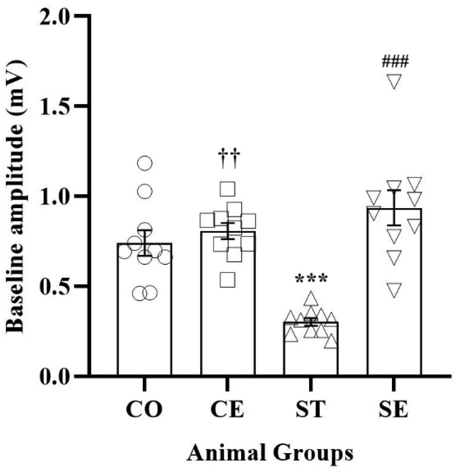
Early-life stress negatively alters mammalian brain programming. Environmental enrichment (EE) has beneficial effects on brain structure and function. This study aimed to evaluate the effects of postnatal environmental enrichment on long-term potentiation (LTP) induction in the hippocampal CA1 area of prenatally stressed female rats. The pregnant Wistar rats were housed in a standard animal room and exposed to traffic noise stress 2 hours/day during the third week of pregnancy. Their offspring either remained intact (ST) or received enrichment (SE) for a month starting from postnatal day 21. The control groups either remained intact (CO) or received enrichment (CE). Basic field excitatory post-synaptic potentials (fEPSPs) were recorded in the CA1 area; then, LTP was induced by high-frequency stimulation. Finally, the serum levels of corticosterone were measured. Our results showed that while the prenatal noise stress decreased the baseline responses of the ST rats when compared to the control rats (P < 0.001), the postnatal EE increased the fEPSPs of both the CE and SE animals when compared to the respective controls. Additionally, high-frequency stimulation (HFS) induced LTP in the fEPSPs of the CO rats (P < 0.001) and failed to induce LTP in the fEPSPs of the ST animals. The enriched condition caused increased potentiation of post-HFS responses in the controls (P < 0.001) and restored the disrupted synaptic plasticity of the CA1 area in the prenatally stressed rats. Likewise, the postnatal EE decreased the elevated serum corticosterone of prenatally stressed offspring (P < 0.001). In conclusion, the postnatal EE restored the stress induced impairment of synaptic plasticity in rats' female offspring.
Citation: Fatemeh Aghighi, Mahmoud Salami, Sayyed Alireza Talaei. Effect of postnatal environmental enrichment on LTP induction in the CA1 area of hippocampus of prenatally traffic noise-stressed female rats[J]. AIMS Neuroscience, 2023, 10(4): 269-281. doi: 10.3934/Neuroscience.2023021
Early-life stress negatively alters mammalian brain programming. Environmental enrichment (EE) has beneficial effects on brain structure and function. This study aimed to evaluate the effects of postnatal environmental enrichment on long-term potentiation (LTP) induction in the hippocampal CA1 area of prenatally stressed female rats. The pregnant Wistar rats were housed in a standard animal room and exposed to traffic noise stress 2 hours/day during the third week of pregnancy. Their offspring either remained intact (ST) or received enrichment (SE) for a month starting from postnatal day 21. The control groups either remained intact (CO) or received enrichment (CE). Basic field excitatory post-synaptic potentials (fEPSPs) were recorded in the CA1 area; then, LTP was induced by high-frequency stimulation. Finally, the serum levels of corticosterone were measured. Our results showed that while the prenatal noise stress decreased the baseline responses of the ST rats when compared to the control rats (P < 0.001), the postnatal EE increased the fEPSPs of both the CE and SE animals when compared to the respective controls. Additionally, high-frequency stimulation (HFS) induced LTP in the fEPSPs of the CO rats (P < 0.001) and failed to induce LTP in the fEPSPs of the ST animals. The enriched condition caused increased potentiation of post-HFS responses in the controls (P < 0.001) and restored the disrupted synaptic plasticity of the CA1 area in the prenatally stressed rats. Likewise, the postnatal EE decreased the elevated serum corticosterone of prenatally stressed offspring (P < 0.001). In conclusion, the postnatal EE restored the stress induced impairment of synaptic plasticity in rats' female offspring.
α amino-3-hydroxy-5-methyl-4-isoxazole propionic acid
brain derived neurotrophic factor
environmental enrichment
field excitatory post-synaptic potentials
glucocorticoid receptors
gamma-Aminobutyric acid
hypothalamic–pituitary–adrenal
high-frequency stimulation
long-term depression
long-term potentiation
N-methyl-D-aspartate
prenatal stress
radioimmunoassay

| [1] |
Zijlmans MA, Riksen-Walraven JM, de Weerth C (2015) Associations between maternal prenatal cortisol concentrations and child outcomes: A systematic review. Neurosci Biobehav R 53: 1-24. https://doi.org/10.1016/j.neubiorev.2015.02.015 
|
| [2] | Barker DJ (1991) The foetal and infant origins of inequalities in health in Britain. J Public Health 13: 64-68. |
| [3] |
Mychasiuk R, Gibb R, Kolb B (2012) Prenatal stress alters dendritic morphology and synaptic connectivity in the prefrontal cortex and hippocampus of developing offspring. Synapse 66: 308-314. https://doi.org/10.1002/syn.21512
|
| [4] |
Zhang H, Shang Y, Xiao X, et al. (2017) Prenatal stress-induced impairments of cognitive flexibility and bidirectional synaptic plasticity are possibly associated with autophagy in adolescent male-offspring. Exp Neurol 298: 68-78. https://doi.org/10.1016/j.expneurol.2017.09.001
|
| [5] |
Weinstock M (2008) The long-term behavioural consequences of prenatal stress. Neurosci Biobehav R 32: 1073-1086. https://doi.org/10.1016/j.neubiorev.2008.03.002
|
| [6] |
Myers RE (1975) Maternal psychological stress and fetal asphyxia: a study in the monkey. Am J Obstet Gynecol 122: 47-59. https://doi.org/10.1016/0002-9378(75)90614-6
|
| [7] | Shapiro ML, Riceberg JS, Seip-Cammack K, et al. (2014) Functional interactions of prefrontal cortex and the hippocampus in learning and memory, in Space, Time and Memory in the Hippocampal Formation. Springer : 517-560. https://doi.org/10.1007/978-3-7091-1292-2_19 |
| [8] |
de los Angeles GAM, del Carmen ROM, Wendy PM, et al. (2016) Tactile stimulation effects on hippocampal neurogenesis and spatial learning and memory in prenatally stressed rats. Brain Res Bull 124: 1-11. https://doi.org/10.1016/j.brainresbull.2016.03.003
|
| [9] |
Andersen N, Krauth N, Nabavi S (2017) Hebbian plasticity in vivo: relevance and induction. Curr Opin Neurobiol 45: 188-192. https://doi.org/10.1016/j.conb.2017.06.001
|
| [10] |
Yeh CM, Huang CC, Hsu KS (2012) Prenatal stress alters hippocampal synaptic plasticity in young rat offspring through preventing the proteolytic conversion of pro-brain-derived neurotrophic factor (BDNF) to mature BDNF. J Physiol 590: 991-1010. https://doi.org/10.1113/jphysiol.2011.222042
|
| [11] |
Girbovan C, Plamondon H (2013) Environmental enrichment in female rodents: considerations in the effects on behavior and biochemical markers. Behav Brain Res 253: 178-190. https://doi.org/10.1016/j.bbr.2013.07.018
|
| [12] |
McCreary JK, Metz GA (2016) Environmental enrichment as an intervention for adverse health outcomes of prenatal stress. Environ Epigenetics 2. https://doi.org/10.1093/eep/dvw013
|
| [13] |
Veena J, Srikumar BN, Mahati K, et al. (2009) Enriched environment restores hippocampal cell proliferation and ameliorates cognitive deficits in chronically stressed rats. J Neurosci Res 87: 831-843. https://doi.org/10.1002/jnr.21907
|
| [14] |
Artola A, Von Frijtag JC, Fermont PCJ, et al. (2006) Long-lasting modulation of the induction of LTD and LTP in rat hippocampal CA1 by behavioural stress and environmental enrichment. Eur J Neurosci 23: 261-272. https://doi.org/10.1111/j.1460-9568.2005.04552.x
|
| [15] |
Segovia G, Del Arco A, De Blas M, et al. (2010) Environmental enrichment increases the in vivo extracellular concentration of dopamine in the nucleus accumbens: a microdialysis study. J Neural Transm 117: 1123-1130. https://doi.org/10.1007/s00702-010-0447-y
|
| [16] |
Montes S, del Carmen Solís-Guillén R, García-Jácome D, et al. (2017) Environmental enrichment reverses memory impairment induced by toluene in mice. Neurotoxicol Teratol 61: 7-16. https://doi.org/10.1016/j.ntt.2017.04.003
|
| [17] |
Nithianantharajah J, Levis H, Murphy M (2004) Environmental enrichment results in cortical and subcortical changes in levels of synaptophysin and PSD-95 proteins. Neurobiol Learn Mem 81: 200-210. https://doi.org/10.1016/j.nlm.2004.02.002
|
| [18] |
Huang FL, Huang K-P, Wu J, et al. (2006) Environmental enrichment enhances neurogranin expression and hippocampal learning and memory but fails to rescue the impairments of neurogranin null mutant mice. J Neurosci 26: 6230-6237. https://doi.org/10.1523/JNEUROSCI.1182-06.2006
|
| [19] |
Tang Y-P, Wang H, Feng R, et al. (2001) Differential effects of enrichment on learning and memory function in NR2B transgenic mice. Neuropharmacology 41: 779-790. https://doi.org/10.1016/S0028-3908(01)00122-8
|
| [20] |
Hellemans KG, Benge LC, Olmstead MC (2004) Adolescent enrichment partially reverses the social isolation syndrome. Dev Brain Res 150: 103-115. https://doi.org/10.1016/j.devbrainres.2004.03.003
|
| [21] |
Dandi E, Kalamari A, Touloumi O, et al. (2018) Beneficial effects of environmental enrichment on behavior, stress reactivity and synaptophysin/BDNF expression in hippocampus following early life stress. Int J Dev Neurosci 67: 19-32. https://doi.org/10.1016/j.ijdevneu.2018.03.003
|
| [22] |
Benito E, Kerimoglu C, Ramachandran B, et al. (2018) RNA-dependent intergenerational inheritance of enhanced synaptic plasticity after environmental enrichment. Cell Rep 23: 546-554. https://doi.org/10.1016/j.celrep.2018.03.059
|
| [23] |
Bhagya VR, Srikumar BN, Veena J, et al. (2017) Short-term exposure to enriched environment rescues chronic stress-induced impaired hippocampal synaptic plasticity, anxiety, and memory deficits. J Neurosci Res 95: 1602-1610. https://doi.org/10.1002/jnr.23992
|
| [24] |
Clemenson GD, Stark SM, Rutledge SM, et al. (2020) Enriching hippocampal memory function in older adults through video games. Behav Brain Res 390: 112667. https://doi.org/10.1016/j.bbr.2020.112667
|
| [25] |
Chang X, Tian Y (2022) Environmental enrichment holds promise as a novel treatment for anesthesia-induced neurocognitive disorders. Neurotoxicol Teratol 94: 107133. https://doi.org/10.1016/j.ntt.2022.107133
|
| [26] |
Barzegar M, Sajjadi FS, Talaei SA, et al. (2015) Prenatal exposure to noise stress: anxiety, impaired spatial memory, and deteriorated hippocampal plasticity in postnatal life. Hippocampus 25: 187-196. https://doi.org/10.1002/hipo.22363
|
| [27] |
Hullinger R, O'Riordan K, Burger C (2015) Environmental enrichment improves learning and memory and long-term potentiation in young adult rats through a mechanism requiring mGluR5 signaling and sustained activation of p70s6k. Neurobiol Learn Mem 125: 126-134. https://doi.org/10.1016/j.nlm.2015.08.006
|
| [28] |
Talaei S, Azami A, Salami M (2016) Postnatal development and sensory experience synergistically underlie the excitatory/inhibitory features of hippocampal neural circuits: glutamatergic and GABAergic neurotransmission. Neuroscience 318: 230-243. https://doi.org/10.1016/j.neuroscience.2016.01.024
|
| [29] |
Yang J, Han H, Cao J, et al. (2006) Prenatal stress modifies hippocampal synaptic plasticity and spatial learning in young rat offspring. Hippocampus 16: 431-436. https://doi.org/10.1002/hipo.20181
|
| [30] |
Alyamani RAS, Murgatroyd C (2018) Epigenetic programming by early-life stress. Prog Mol Biol Transl 157: 133-150. https://doi.org/10.1016/bs.pmbts.2018.01.004
|
| [31] |
Jafari Z, Mehla J, Kolb BE, et al. (2017) Prenatal noise stress impairs HPA axis and cognitive performance in mice. Sci Rep 7: 1-13. https://doi.org/10.1038/s41598-017-09799-6
|
| [32] |
Szuran TF, Pliška V, Pokorny J, et al. (2000) Prenatal stress in rats: effects on plasma corticosterone, hippocampal glucocorticoid receptors, and maze performance. Physiol Behav 71: 353-362. https://doi.org/10.1016/S0031-9384(00)00351-6
|
| [33] |
Mifsud KR, Saunderson EA, Spiers H, et al. (2017) Rapid down-regulation of glucocorticoid receptor gene expression in the dentate gyrus after acute stress in vivo: role of DNA methylation and microRNA activity. Neuroendocrinology 104: 157-169. https://doi.org/10.1159/000445875
|
| [34] |
Herman JP, Spencer R (1998) Regulation of hippocampal glucocorticoid receptor gene transcription and protein expression in vivo. J Neurosci 18: 7462-7473. https://doi.org/10.1523/JNEUROSCI.18-18-07462.1998
|
| [35] |
Henry C, Kabbaj M, Simon H, et al. (1994) Prenatal stress increases the hypothalamo-pituitary-adrenal axis response in young and adult rats. J Neuroendocrinol 6: 341-345. https://doi.org/10.1111/j.1365-2826.1994.tb00591.x
|
| [36] |
Harris A, Seckl J (2011) Glucocorticoids, prenatal stress and the programming of disease. Horm Behav 59: 279-289. https://doi.org/10.1016/j.yhbeh.2010.06.007
|
| [37] |
Mandyam CD, Crawford EF, Eisch AJ, et al. (2008) Stress experienced in utero reduces sexual dichotomies in neurogenesis, microenvironment, and cell death in the adult rat hippocampus. Dev Neurobiol 68: 575-589. https://doi.org/10.1002/dneu.20600
|
| [38] |
Badihian N, Daniali SS, Kelishadi R (2019) Transcriptional and epigenetic changes of brain derived neurotrophic factor following prenatal stress: A systematic review of animal studies. Neurosci Biobehav Rev 117: 211-231. https://doi.org/10.1016/j.neubiorev.2019.12.018
|
| [39] |
Tavassoli E, Saboory E, Teshfam M, et al. (2013) Effect of prenatal stress on density of NMDA receptors in rat brain. Int J Dev Neurosci 31: 790-795. https://doi.org/10.1016/j.ijdevneu.2013.09.010
|
| [40] |
Sun H, Guan L, Zhu Z, et al. (2013) Reduced levels of NR1 and NR2A with depression-like behavior in different brain regions in prenatally stressed juvenile offspring. PLOS ONE 8: e81775. https://doi.org/10.1371/journal.pone.0081775
|
| [41] |
Lu Y, Zhang J, Zhang L, et al. (2017) Hippocampal Acetylation may Improve Prenatal-Stress-Induced Depression-Like Behavior of Male Offspring Rats Through Regulating AMPARs Expression. Neurochem Res 42: 3456-3464. https://doi.org/10.1007/s11064-017-2393-7
|
| [42] |
Hu L, Han B, Zhao X, et al. (2016) Chronic early postnatal scream sound stress induces learning deficits and NMDA receptor changes in the hippocampus of adult mice. Neuroreport 27: 397-403. https://doi.org/10.1097/WNR.0000000000000552
|
| [43] |
Fang Y, Li H, Chang L, et al. (2018) Prenatal stress induced gender-specific alterations of N-methyl-d-aspartate receptor subunit expression and response to Abeta in offspring hippocampal cells. Behav Brain Res 336: 182-190. https://doi.org/10.1016/j.bbr.2017.08.036
|
| [44] |
Adrover E, Pallarés ME, Baier CJ, et al. (2015) Glutamate neurotransmission is affected in prenatally stressed offspring. Neurochem Int 88: 73-87. https://doi.org/10.1016/j.neuint.2015.05.005
|
| [45] |
Lau PY-P, Katona L, Saghy P, et al. (2017) Long-term plasticity in identified hippocampal GABAergic interneurons in the CA1 area in vivo. Brain Struct Funct 222: 1809-1827. https://doi.org/10.1007/s00429-016-1309-7
|
| [46] |
Hu W, Zhang M, Czéh B, et al. (2010) Stress impairs GABAergic network function in the hippocampus by activating nongenomic glucocorticoid receptors and affecting the integrity of the parvalbumin-expressing neuronal network. Neuropsychopharmacology 35: 1693-1707. https://doi.org/10.1038/npp.2010.31
|
| [47] |
Veerawatananan B, Surakul P, Chutabhakdikul N (2016) Maternal restraint stress delays maturation of cation-chloride cotransporters and GABAA receptor subunits in the hippocampus of rat pups at puberty. Neurobiol Stress 3: 1-7. https://doi.org/10.1016/j.ynstr.2015.12.001
|
| [48] |
Lussier SJ, Stevens HE (2016) Delays in GABAergic interneuron development and behavioral inhibition after prenatal stress. Dev Neurobiol 76: 1078-1091. https://doi.org/10.1002/dneu.22376
|
| [49] |
Tang AC, Zou B (2002) Neonatal exposure to novelty enhances long-term potentiation in CA1 of the rat hippocampus. Hippocampus 12: 398-404. https://doi.org/10.1002/hipo.10017
|
| [50] |
Yang J, Hou C, Ma N, et al. (2007) Enriched environment treatment restores impaired hippocampal synaptic plasticity and cognitive deficits induced by prenatal chronic stress. Neurobiol Learn Mem 87: 257-263. https://doi.org/10.1016/j.nlm.2006.09.001
|
| [51] |
Van Praag H, Kempermann G, Gage FH (2000) Neural consequences of enviromental enrichment. Nat Rev Neurosci 1: 191-198. https://doi.org/10.1038/35044558
|
| [52] |
Lee EH, Hsu WL, Ma YL, et al. (2003) Enrichment enhances the expression of sgk, a glucocorticoid-induced gene, and facilitates spatial learning through glutamate AMPA receptor mediation. Eur J Neurosci 18: 2842-2852. https://doi.org/10.1111/j.1460-9568.2003.03032.x
|
| [53] |
Hullinger R, O'Riordan K, Burger C (2015) Environmental enrichment improves learning and memory and long-term potentiation in young adult rats through a mechanism requiring mGluR5 signaling and sustained activation of p70s6k. Neurobiol Learn Mem 125: 126-134. https://doi.org/10.1016/j.nlm.2015.08.006
|
| [54] |
Begenisic T, Spolidoro M, Braschi C, et al. (2011) Environmental enrichment decreases GABAergic inhibition and improves cognitive abilities, synaptic plasticity, and visual functions in a mouse model of Down syndrome. Front Cell Neurosci 5: 29. https://doi.org/10.3389/fncel.2011.00029
|
| [55] |
Novaes LS, dos Santos NB, Batalhote RFP, et al. (2017) Environmental enrichment protects against stress-induced anxiety: Role of glucocorticoid receptor, ERK, and CREB signaling in the basolateral amygdala. Neuropharmacology 113: 457-466. https://doi.org/10.1016/j.neuropharm.2016.10.026
|
| [56] |
Dandi E, Kalamari A, Touloumi O, et al. (2018) Beneficial effects of environmental enrichment on behavior, stress reactivity and synaptophysin/BDNF expression in hippocampus following early life stress. Int J Dev Neurosci 67: 19-32. https://doi.org/10.1016/j.ijdevneu.2018.03.003
|


Figures(3)

Fatemeh Aghighi, Mahmoud Salami, Sayyed Alireza Talaei. Effect of postnatal environmental enrichment on LTP induction in the CA1 area of hippocampus of prenatally traffic noise-stressed female rats[J]. AIMS Neuroscience, 2023, 10(4): 269-281. doi: 10.3934/Neuroscience.2023021


 DownLoad: