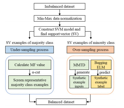
To handle imbalanced datasets in machine learning or deep learning models, some studies suggest sampling techniques to generate virtual examples of minority classes to improve the models' prediction accuracy. However, for kernel-based support vector machines (SVM), some sampling methods suggest generating synthetic examples in an original data space rather than in a high-dimensional feature space. This may be ineffective in improving SVM classification for imbalanced datasets. To address this problem, we propose a novel hybrid sampling technique termed modified mega-trend-diffusion-extreme learning machine (MMTD-ELM) to effectively move the SVM decision boundary toward a region of the majority class. By this movement, the prediction of SVM for minority class examples can be improved. The proposed method combines α-cut fuzzy number method for screening representative examples of majority class and MMTD method for creating new examples of the minority class. Furthermore, we construct a bagging ELM model to monitor the similarity between new examples and original data. In this paper, four datasets are used to test the efficiency of the proposed MMTD-ELM method in imbalanced data prediction. Additionally, we deployed two SVM models to compare prediction performance of the proposed MMTD-ELM method with three state-of-the-art sampling techniques in terms of geometric mean (G-mean), F-measure (F1), index of balanced accuracy (IBA) and area under curve (AUC) metrics. Furthermore, paired t-test is used to elucidate whether the suggested method has statistically significant differences from the other sampling techniques in terms of the four evaluation metrics. The experimental results demonstrated that the proposed method achieves the best average values in terms of G-mean, F1, IBA and AUC. Overall, the suggested MMTD-ELM method outperforms these sampling methods for imbalanced datasets.
Citation: Liang-Sian Lin, Chen-Huan Kao, Yi-Jie Li, Hao-Hsuan Chen, Hung-Yu Chen. Improved support vector machine classification for imbalanced medical datasets by novel hybrid sampling combining modified mega-trend-diffusion and bagging extreme learning machine model[J]. Mathematical Biosciences and Engineering, 2023, 20(10): 17672-17701. doi: 10.3934/mbe.2023786
To handle imbalanced datasets in machine learning or deep learning models, some studies suggest sampling techniques to generate virtual examples of minority classes to improve the models' prediction accuracy. However, for kernel-based support vector machines (SVM), some sampling methods suggest generating synthetic examples in an original data space rather than in a high-dimensional feature space. This may be ineffective in improving SVM classification for imbalanced datasets. To address this problem, we propose a novel hybrid sampling technique termed modified mega-trend-diffusion-extreme learning machine (MMTD-ELM) to effectively move the SVM decision boundary toward a region of the majority class. By this movement, the prediction of SVM for minority class examples can be improved. The proposed method combines α-cut fuzzy number method for screening representative examples of majority class and MMTD method for creating new examples of the minority class. Furthermore, we construct a bagging ELM model to monitor the similarity between new examples and original data. In this paper, four datasets are used to test the efficiency of the proposed MMTD-ELM method in imbalanced data prediction. Additionally, we deployed two SVM models to compare prediction performance of the proposed MMTD-ELM method with three state-of-the-art sampling techniques in terms of geometric mean (G-mean), F-measure (F1), index of balanced accuracy (IBA) and area under curve (AUC) metrics. Furthermore, paired t-test is used to elucidate whether the suggested method has statistically significant differences from the other sampling techniques in terms of the four evaluation metrics. The experimental results demonstrated that the proposed method achieves the best average values in terms of G-mean, F1, IBA and AUC. Overall, the suggested MMTD-ELM method outperforms these sampling methods for imbalanced datasets.

| [1] |
Q. Wang, W. Cao, J. Guo, J. Ren, Y. Cheng, D. N. Davis, DMP_MI: An effective diabetes mellitus classification algorithm on imbalanced data with missing values, IEEE Access, 7 (2019), 102232–102238. https://doi.org/10.1109/ACCESS.2019.2929866 doi: 10.1109/ACCESS.2019.2929866

|
| [2] |
L. Yousefi, S. Swift, M. Arzoky, L. Saachi, L. Chiovato, A. Tucker, Opening the black box: Personalizing type 2 diabetes patients based on their latent phenotype and temporal associated complication rules, Comput. Intell., 37 (2021), 1460–1498. https://doi.org/10.1111/coin.12313 doi: 10.1111/coin.12313
|
| [3] |
B. Krawczyk, M. Galar, Ł. Jeleń, F. Herrera, Evolutionary undersampling boosting for imbalanced classification of breast cancer malignancy, Appl. Soft. Comput., 38 (2016), 714–726. https://doi.org/10.1016/j.asoc.2015.08.060 doi: 10.1016/j.asoc.2015.08.060
|
| [4] |
A. K. Mishra, P. Roy, S. Bandyopadhyay, S. K. Das, Breast ultrasound tumour classification: A machine learning-radiomics based approach, Expert Syst., 38 (2021), 12713. https://doi.org/10.1111/exsy.12713 doi: 10.1111/exsy.12713
|
| [5] |
J. Zhou, X. Li, Y. Ma, Z. Wu, Z. Xie, Y. Zhang, et al., Optimal modeling of anti-breast cancer candidate drugs screening based on multi-model ensemble learning with imbalanced data, Math. Biosci. Eng., 20 (2023), 5117–5134. https://doi.org/10.3934/mbe.2023237 doi: 10.3934/mbe.2023237
|
| [6] |
L. Zhang, H. Yang, Z. Jiang, Imbalanced biomedical data classification using self-adaptive multilayer ELM combined with dynamic GAN, Biomed. Eng. Online, 17 (2018), 1–21. https://doi.org/10.1186/s12938-018-0604-3 doi: 10.1186/s12938-018-0604-3
|
| [7] |
H. S. Basavegowda, G. Dagnew, Deep learning approach for microarray cancer data classification, CAAI Trans. Intell. Technol., 5 (2020), 22–33. https://doi.org/10.1049/trit.2019.0028 doi: 10.1049/trit.2019.0028
|
| [8] |
B. Pes, Learning from high-dimensional biomedical datasets: the issue of class Imbalance, IEEE Access, 8 (2020), 13527–13540. https://doi.org/10.1109/ACCESS.2020.2966296 doi: 10.1109/ACCESS.2020.2966296
|
| [9] |
J. Wang, Prediction of postoperative recovery in patients with acoustic neuroma using machine learning and SMOTE-ENN techniques, Math. Biosci. Eng., 19 (2022), 10407–10423. https://doi.org/10.3934/mbe.2022487 doi: 10.3934/mbe.2022487
|
| [10] |
V. Babar, R. Ade, A novel approach for handling imbalanced data in medical diagnosis using undersampling technique, Commun. Appl. Electron., 5 (2016), 36–42. https://doi.org/10.5120/cae2016652323 doi: 10.5120/cae2016652323
|
| [11] |
J. Zhang, L. Chen, F. Abid, Prediction of breast cancer from imbalance respect using cluster-based undersampling method, J. Healthcare Eng., 2019 (2019), 7294582. https://doi.org/10.1155/2019/7294582 doi: 10.1155/2019/7294582
|
| [12] | P. Vuttipittayamongkol, E. Elyan, Overlap-based undersampling method for classification of imbalanced medical datasets, in IFIP International Conference on Artificial Intelligence Applications and Innovations, (2020), 358–369. https://doi.org/10.1007/978-3-030-49186-4_30 |
| [13] |
N. V. Chawla, K. W. Bowyer, L. O. Hall, W. P. Kegelmeyer, SMOTE: Synthetic minority over-sampling technique, J. Artif. Intell. Res., 16 (2002), 321–357. https://doi.org/10.1613/jair.953 doi: 10.1613/jair.953
|
| [14] | C. Bunkhumpornpat, K. Sinapiromsaran, C. Lursinsap, Safe-Level-SMOTE: Safe-level-synthetic minority over-sampling technique for handling the class imbalanced problem, in Pacific-Asia Conference on Knowledge Discovery and Data Mining, 5476 (2009), 475–482. https://doi.org/10.1007/978-3-642-01307-2_43 |
| [15] | D. A. Cieslak, N. V. Chawla, A. Striegel, Combating imbalance in network intrusion datasets, in 2006 IEEE International Conference on Granular Computing, (2006), 732–737. https://doi.org/10.1109/GRC.2006.1635905 |
| [16] | J. de la Calleja, O. Fuentes, J. González, Selecting minority examples from misclassified data for over-sampling, in Proceedings of the Twenty-First International Florida Artificial Intelligence Research Society Conference, (2008), 276–281. |
| [17] |
M. A. H. Farquad, I. Bose, Preprocessing unbalanced data using support vector machine, Decis. Support Syst., 53 (2012), 226–233. https://doi.org/10.1016/j.dss.2012.01.016 doi: 10.1016/j.dss.2012.01.016
|
| [18] |
Q. Wang, A hybrid sampling SVM approach to imbalanced data classification, Abstr. Appl. Anal., 2014 (2014), 972786. https://doi.org/10.1155/2014/972786 doi: 10.1155/2014/972786
|
| [19] |
J. Zhang, L. Chen, Clustering-based undersampling with random over sampling examples and support vector machine for imbalanced classification of breast cancer diagnosis, Comput. Assisted Surg., 24 (2019), 62–72. https://doi.org/10.1080/24699322.2019.1649074 doi: 10.1080/24699322.2019.1649074
|
| [20] |
D. Li, C. Wu, T. Tsai, Y. Lina, Using mega-trend-diffusion and artificial samples in small data set learning for early flexible manufacturing system scheduling knowledge, Comput. Oper. Res., 34 (2007), 966–982. https://doi.org/10.1016/j.cor.2005.05.019 doi: 10.1016/j.cor.2005.05.019
|
| [21] |
L. Breiman, Bagging predictors, Mach. Learn., 24 (1996), 123–140. https://doi.org/10.1007/BF00058655 doi: 10.1007/BF00058655
|
| [22] |
J. Alcalá-Fdez, L. Sánchez, S. García, M. J. del Jesus, S. Ventura, J. M. Garrell, et al., KEEL: a software tool to assess evolutionary algorithms for data mining problems, Soft Comput., 13 (2009), 307–318. https://doi.org/10.1007/s00500-008-0323-y doi: 10.1007/s00500-008-0323-y
|
| [23] | B. Haznedar, M.T. Arslan, A. Kalinli, Microarray Gene Expression Cancer Data, 2017. Available from: https://doi.org/10.17632/YNM2tst2hh.4. |
| [24] |
M. Kubat, R. C. Holte, S. Matwin, Machine learning for the detection of oil spills in satellite radar images, Mach. Learn., 30 (1998), 195–215. https://doi.org/10.1023/A:1007452223027 doi: 10.1023/A:1007452223027
|
| [25] | V. García, R. A. Mollineda, J. S. Sánchez, Theoretical analysis of a performance measure for imbalanced data, in 2010 20th International Conference on Pattern Recognition, (2010), 617–620. https://doi.org/10.1109/ICPR.2010.156 |
| [26] |
J. A. Hanley, B. J. McNeil, The meaning and use of the area under a receiver operating characteristic (ROC) curve, Radiology, 143 (1982), 29–36. https://doi.org/10.1148/radiology.143.1.7063747 doi: 10.1148/radiology.143.1.7063747
|
| [27] |
C. Cortes, V. Vapnik, Support-vector networks, Mach. Learn., 20 (1995), 273–297. https://doi.org/10.1007/BF00994018 doi: 10.1007/BF00994018
|
| [28] |
C. Liu, T. Lin, K. Yuan, P. Chiueh, Spatio-temporal prediction and factor identification of urban air quality using support vector machine, Urban Clim., 41 (2022), 101055. https://doi.org/10.1016/j.uclim.2021.101055 doi: 10.1016/j.uclim.2021.101055
|
| [29] |
Z. Wang, Y. Yang, S. Yue, Air quality classification and measurement based on double output vision transformer, IEEE Internet Things J., 9 (2022), 20975–20984. https://doi.org/10.1109/JIOT.2022.3176126 doi: 10.1109/JIOT.2022.3176126
|
| [30] |
L. Wei, Q. Gan, T. Ji, Cervical cancer histology image identification method based on texture and lesion area features, Comput. Assisted Surg., 22 (2017), 186–199. https://doi.org/10.1080/24699322.2017.1389397 doi: 10.1080/24699322.2017.1389397
|
| [31] |
I. Izonin, R. Tkachenko, O. Gurbych, M. Kovac, L. Rutkowski, R. Holoven, A non-linear SVR-based cascade model for improving prediction accuracy of biomedical data analysis, Math. Biosci. Eng., 20 (2023), 13398–13414. https://doi.org/10.3934/mbe.2023597 doi: 10.3934/mbe.2023597
|
| [32] |
G. C. Batista, D. L. Oliveira, O. Saotome, W. L. S. Silva, A low-power asynchronous hardware implementation of a novel SVM classifier, with an application in a speech recognition system, Microelectron. J., 105 (2020), 104907. https://doi.org/10.1016/j.mejo.2020.104907 doi: 10.1016/j.mejo.2020.104907
|
| [33] |
A. A. Viji, J. Jasper, T. Latha, Efficient emotion based automatic speech recognition using optimal deep learning approach, Optik, (2022), 170375. https://doi.org/10.1016/j.ijleo.2022.170375 doi: 10.1016/j.ijleo.2022.170375
|
| [34] | Z. Zeng, J. Gao, Improving SVM classification with imbalance data set, in International Conference on Neural Information Processing, 5863 (2009), 389–398. https://doi.org/10.1007/978-3-642-10677-4_44 |
| [35] |
Z. Luo, H. Parvïn, H. Garg, S. N. Qasem, K. Pho, Z. Mansor, Dealing with imbalanced dataset leveraging boundary samples discovered by support vector data description, Comput. Mater. Continua, 66 (2021), 2691–2708. https://doi.org/10.32604/cmc.2021.012547 doi: 10.32604/cmc.2021.012547
|
| [36] |
G. Huang, Q. Zhu, C. Siew, Extreme learning machine: Theory and applications, Neurocomputing, 70 (2006), 489–501. https://doi.org/10.1016/j.neucom.2005.12.126 doi: 10.1016/j.neucom.2005.12.126
|
| [37] | F. Pedregosa, G. Varoquaux, A. Gramfort, V. Michel, B. Thirion, O. Grisel, et al., Scikit-learn: Machine learning in Python, J. Mach. Learn. Res., 12 (2011), 2825–2830 |
| [38] |
C. Wu, L. Chen, A model with deep analysis on a large drug network for drug classification, Math. Biosci. Eng., 20 (2023), 383–401. https://doi.org/10.3934/mbe.2023018 doi: 10.3934/mbe.2023018
|
Figures(10) / Tables(16)

Liang-Sian Lin, Chen-Huan Kao, Yi-Jie Li, Hao-Hsuan Chen, Hung-Yu Chen. Improved support vector machine classification for imbalanced medical datasets by novel hybrid sampling combining modified mega-trend-diffusion and bagging extreme learning machine model[J]. Mathematical Biosciences and Engineering, 2023, 20(10): 17672-17701. doi: 10.3934/mbe.2023786


 DownLoad: