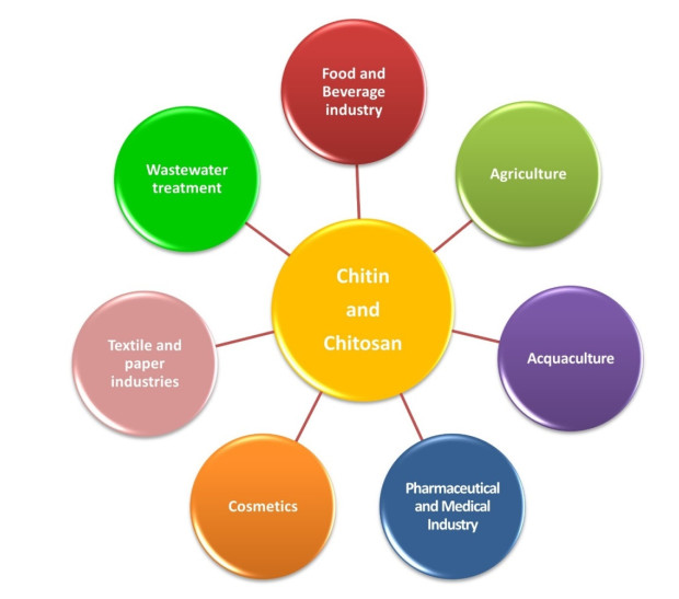
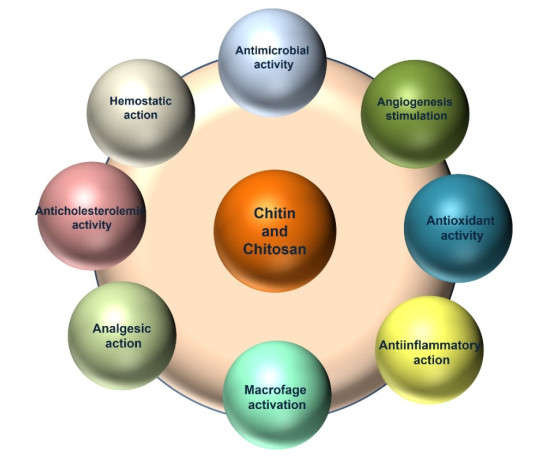
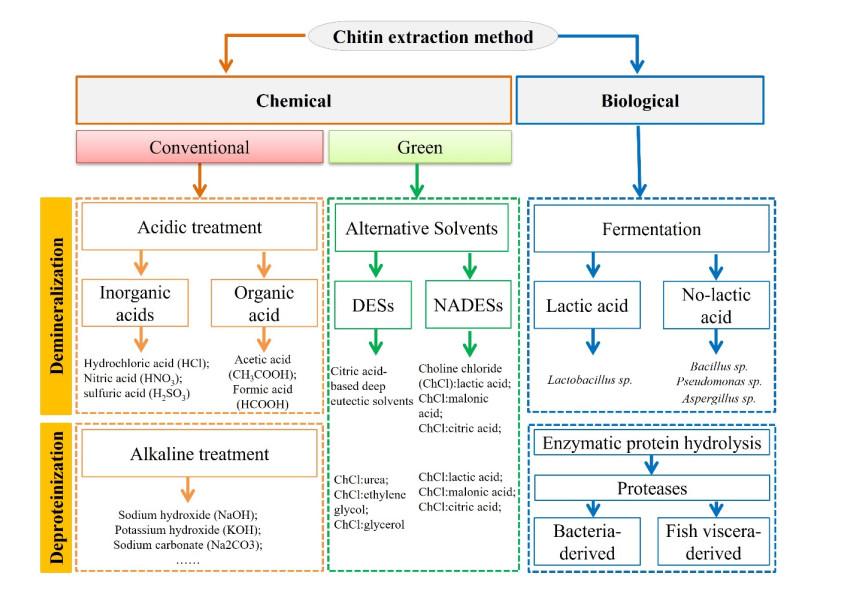
Chitin is the second most plentiful natural biomass after cellulose, with a yearly production of about 1 × 10¹⁰–1 × 10¹² tonnes. It can be obtained mainly from sea crustaceans' shells, containing 15–40% chitin. Full or partial deacetylation of chitin generates chitosan. Chitin and chitosan are used in several industrial sectors, as they exhibit high biocompatibility, biodegradability and several biological functions (e.g., antioxidant, antimicrobial and antitumoral activities). These biopolymers' market trends are destined to grow in the coming years, confirming their relevance. As a result, low-cost and industrial-scale production is the main challenge. Scientific literature reports two major technologies for chitin and chitosan recovery from crustacean waste: chemical and biological methods. The chemical treatment can be performed using conventional solvents, typically strong acid and alkaline solutions, or alternative green solvents, such as deep eutectic solvents (DESs) and natural deep eutectic solvents (NADESs). Biological methods use enzymatic or fermentation processes. For each route, this paper reviews the advantages and drawbacks in terms of environmental and economic sustainability. The conventional chemical method is still the most used but results in high environmental impacts. Green chemical methods by DESs and NADESs use low-toxic and biodegradable solvents but require high temperatures and long reaction times. Biological methods are eco-friendly but have limitations in the upscaling process, and are affected by high costs and long reaction times. This review focuses on the methodologies available to isolate chitin from crustaceans, providing a comprehensive overview. At the same time, it examines the chemical, biological and functional properties of chitin and its derivative, along with their most common applications. Consequently, this work represents a valuable knowledge tool for selecting and developing the most suitable and effective technologies to produce chitin and its derivatives.
Citation: Alessandra Verardi, Paola Sangiorgio, Stefania Moliterni, Simona Errico, Anna Spagnoletta, Salvatore Dimatteo. Advanced technologies for chitin recovery from crustacean waste[J]. Clean Technologies and Recycling, 2023, 3(1): 4-43. doi: 10.3934/ctr.2023002
Chitin is the second most plentiful natural biomass after cellulose, with a yearly production of about 1 × 10¹⁰–1 × 10¹² tonnes. It can be obtained mainly from sea crustaceans' shells, containing 15–40% chitin. Full or partial deacetylation of chitin generates chitosan. Chitin and chitosan are used in several industrial sectors, as they exhibit high biocompatibility, biodegradability and several biological functions (e.g., antioxidant, antimicrobial and antitumoral activities). These biopolymers' market trends are destined to grow in the coming years, confirming their relevance. As a result, low-cost and industrial-scale production is the main challenge. Scientific literature reports two major technologies for chitin and chitosan recovery from crustacean waste: chemical and biological methods. The chemical treatment can be performed using conventional solvents, typically strong acid and alkaline solutions, or alternative green solvents, such as deep eutectic solvents (DESs) and natural deep eutectic solvents (NADESs). Biological methods use enzymatic or fermentation processes. For each route, this paper reviews the advantages and drawbacks in terms of environmental and economic sustainability. The conventional chemical method is still the most used but results in high environmental impacts. Green chemical methods by DESs and NADESs use low-toxic and biodegradable solvents but require high temperatures and long reaction times. Biological methods are eco-friendly but have limitations in the upscaling process, and are affected by high costs and long reaction times. This review focuses on the methodologies available to isolate chitin from crustaceans, providing a comprehensive overview. At the same time, it examines the chemical, biological and functional properties of chitin and its derivative, along with their most common applications. Consequently, this work represents a valuable knowledge tool for selecting and developing the most suitable and effective technologies to produce chitin and its derivatives.

| [1] |
Pighinelli L (2019) Methods of chitin production a short review. Am J Biomed Sci Res 3: 307–314. https://doi.org/10.34297/AJBSR.2019.03.000682 doi: 10.34297/AJBSR.2019.03.000682

|
| [2] | Research and Markets, Chitin and Chitosan Derivatives: Global Strategic Business Report. Research and Markets, 2022. Available from: https://www.researchandmarkets.com/reports/338576/chitin_and_chitosan_derivatives_global_strategic#: ~: text = In%20the%20changed%20post%20COVID-19%20business%20landscape%2C%20the, CAGR%20of%2018.4%25%20over%20the%20analysis%20period%202020-2027. |
| [3] |
Ahmad SI, Ahmad R, Khan MS, et al. (2020) Chitin and its derivatives: Structural properties and biomedical applications. Int J Biol Macromol 164: 526–539. https://doi.org/10.1016/j.ijbiomac.2020.07.098 doi: 10.1016/j.ijbiomac.2020.07.098
|
| [4] |
Aranaz I, Alcántara AR, Civera MC, et al. (2021) Chitosan: An overview of its properties and applications. Polymers 13: 3256. https://doi.org/10.3390/polym13193256 doi: 10.3390/polym13193256
|
| [5] |
Islam N, Hoque M, Taharat SF (2023) Recent advances in extraction of chitin and chitosan. World J Microbiol Biotechnol 39: 28. https://doi.org/10.1007/s11274-022-03468-1 doi: 10.1007/s11274-022-03468-1
|
| [6] | Crini G (2019) Historical landmarks in the discovery of chitin, In: Crini G, Lichtfouse E, Sustainable Agriculture Reviews 35, 1 Ed., Cham: Springer, 1–47. https://doi.org/10.1007/978-3-030-16538-3_1 |
| [7] |
Iber BT, Kasan NA, Torsabo D, et al. (2022) A review of various sources of chitin and chitosan in nature. J Renew Mater 10: 1097. https://doi.org/10.32604/jrm.2022.018142 doi: 10.32604/jrm.2022.018142
|
| [8] | Broek LA, Boeriu CG, Stevens CV (2019) Chitin and Chitosan: Properties and Applications, Hoboken: Wiley. https://doi.org/10.1002/9781119450467 |
| [9] |
El Knidri H, Belaabed R, Addaou A, et al. (2018) Extraction, chemical modification and characterization of chitin and chitosan. Int J Biol Macromol 120: 1181–1189. https://doi.org/10.1016/j.ijbiomac.2018.08.139 doi: 10.1016/j.ijbiomac.2018.08.139
|
| [10] | Sawada D, Nishiyama Y, Langan P, et al. (2012) Water in crystalline fibers of dihydrate β-chitin results in unexpected absence of intramolecular hydrogen bonding. PLoS One 7: e39376. https://doi.org/10.1371/journal.pone.0039376 |
| [11] |
Abidin NAZ, Kormin F, Abidin NAZ, et al. (2020) The potential of insects as alternative sources of chitin: An overview on the chemical method of extraction from various sources. Int J Mol Sci 21: 1–25. https://doi.org/10.3390/ijms21144978 doi: 10.3390/ijms21144978
|
| [12] |
Hahn T, Roth A, Ji R, et al. (2020) Chitosan production with larval exoskeletons derived from the insect protein production. J Biotechnol 310: 62–67. https://doi.org/10.1016/j.jbiotec.2019.12.015 doi: 10.1016/j.jbiotec.2019.12.015
|
| [13] | FAO, The State of World Fisheries and Aquaculture 2020. Sustainability in Action. FAO, 2020. Available from: https://doi.org/10.4060/ca9229en. |
| [14] |
Kurita K (2006) Chitin and chitosan: Functional biopolymers from marine crustaceans. Marine Biotechnol 8: 203–226. https://doi.org/10.1007/s10126-005-0097-5 doi: 10.1007/s10126-005-0097-5
|
| [15] | Özogul F, Hamed I, Özogul Y, et al. (2018) Crustacean by-products, In: Varelis P, Melton L, Shahidi F, Encyclopedia of Food Chemistry, Amsterdam: Elsevier, 33–38. https://doi.org/10.1016/B978-0-08-100596-5.21690-9 |
| [16] | Bastiaens L, Soetemans L, D'Hondt E, et al. (2019) Sources of chitin and chitosan and their isolation, In Broek LA, Boeriu CG, Stevens CV, Chitin and Chitosan: Properties and Applications, 1 Ed., Amsterdam: Elsevier, 1–34. https://doi.org/10.1002/9781119450467.ch1 |
| [17] |
Jones M, Kujundzic M, John S, et al. (2020) Crab vs. mushroom: A review of crustacean and fungal chitin in wound treatment. Mar Drugs 18: 64. https://doi.org/10.3390/md18010064 doi: 10.3390/md18010064
|
| [18] |
Arbia W, Arbia L, Adour L, et al. (2013) Chitin extraction from crustacean shells using biological methods—A review. Food Hydrocolloid 31: 392–403. https://doi.org/10.1016/j.foodhyd.2012.10.025 doi: 10.1016/j.foodhyd.2012.10.025
|
| [19] | Chakravarty J, Yang CL, Palmer J, et al. (2018) Chitin extraction from lobster shell waste using microbial culture-based methods. Appl Food Biotechnol 5: 141–154. |
| [20] |
Maddaloni M, Vassalini I, Alessandri I (2020) Green routes for the development of chitin/chitosan sustainable hydrogels. Sustain Chem 1: 325–344. https://doi.org/10.3390/suschem1030022 doi: 10.3390/suschem1030022
|
| [21] |
Kozma M, Acharya B, Bissessur R (2022) Chitin, chitosan, and nanochitin: Extraction, synthesis, and applications. Polymers 14: 3989. https://doi.org/10.3390/polym14193989 doi: 10.3390/polym14193989
|
| [22] | Morin-Crini N, Lichtfouse E, Torri G, et al. (2019) Fundamentals and applications of chitosan, In: Crini G, Lichtfouse E, Sustainable Agriculture Reviews 35, 1 Ed., Cham: Springer, 49–123. https://doi.org/10.1007/978-3-030-16538-3_2 |
| [23] |
Arnold ND, Brück WM, Garbe D, et al. (2020) Enzymatic modification of native chitin and conversion to specialty chemical products. Mar Drugs 18: 93. https://doi.org/10.3390/md18020093 doi: 10.3390/md18020093
|
| [24] |
Fernando LD, Widanage MCD, Penfield J, et al. (2021) Structural polymorphism of chitin and chitosan in fungal cell walls from solid-state NMR and principal component analysis. Front Mol Biosci 8: 727053. https://doi.org/10.3389/fmolb.2021.727053 doi: 10.3389/fmolb.2021.727053
|
| [25] |
Kaya M, Mujtaba M, Ehrlich H, et al. (2017) On chemistry of γ-chitin. Carbohyd Polym 176: 177–186. https://doi.org/10.1016/j.carbpol.2017.08.076 doi: 10.1016/j.carbpol.2017.08.076
|
| [26] |
Cao S, Liu Y, Shi L, et al. (2022) N-Acetylglucosamine as a platform chemical produced from renewable resources: opportunity, challenge, and future prospects. Green Chem 24: 493–509. https://doi.org/10.1039/D1GC03725K doi: 10.1039/D1GC03725K
|
| [27] |
de Queiroz Antonino RSCM, Fook BRPL, de Oliveira Lima VA, et al. (2017) Preparation and characterization of chitosan obtained from shells of shrimp (Litopenaeus vannamei Boone). Mar Drugs 15: 141. https://doi.org/10.3390/md15050141 doi: 10.3390/md15050141
|
| [28] |
Yu Z, Lau D (2017) Flexibility of backbone fibrils in α-chitin crystals with different degree of acetylation. Carbohyd Polym 174: 941–947. https://doi.org/10.1016/j.carbpol.2017.06.099 doi: 10.1016/j.carbpol.2017.06.099
|
| [29] |
Philibert T, Lee BH, Fabien N (2017) Current status and new perspectives on chitin and chitosan as functional biopolymers. Appl Biochem Biotech 181: 1314–1337. https://doi.org/10.1007/s12010-016-2286-2 doi: 10.1007/s12010-016-2286-2
|
| [30] |
Philippova OE, Korchagina EV, Volkov EV, et al. (2012) Aggregation of some water-soluble derivatives of chitin in aqueous solutions: Role of the degree of acetylation and effect of hydrogen bond breaker. Carbohyd Polym 87: 687–694. https://doi.org/10.1016/j.carbpol.2011.08.043 doi: 10.1016/j.carbpol.2011.08.043
|
| [31] |
Younes I, Sellimi S, Rinaudo M, et al. (2014) Influence of acetylation degree and molecular weight of homogeneous chitosans on antibacterial and antifungal activities. Int J Food Microbiol 185: 57–63. https://doi.org/10.1016/j.ijfoodmicro.2014.04.029 doi: 10.1016/j.ijfoodmicro.2014.04.029
|
| [32] |
Hattori H, Ishihara M (2015) Changes in blood aggregation with differences in molecular weight and degree of deacetylation of chitosan. Biomed Mater 10: 015014. https://doi.org/10.1088/1748-6041/10/1/015014 doi: 10.1088/1748-6041/10/1/015014
|
| [33] |
Mourya VK, Inamdar NN, Choudhari YM (2011) Chitooligosaccharides: Synthesis, characterization and applications. Polym Sci Ser A+ 53: 583–612. https://doi.org/10.1134/S0965545X11070066 doi: 10.1134/S0965545X11070066
|
| [34] |
Errico S, Spagnoletta A, Verardi A, et al. (2022) Tenebrio molitor as a source of interesting natural compounds, their recovery processes, biological effects, and safety aspects. Compr Rev Food Sci Food Saf 21: 148–197. https://doi.org/10.1111/1541-4337.12863 doi: 10.1111/1541-4337.12863
|
| [35] | Elieh-Ali-Komi D, Hamblin MR (2016) Chitin and chitosan: Production and application of versatile biomedical nanomaterials. Int J Adv Res 4: 411–427. |
| [36] |
Liang S, Sun Y, Dai X (2018) A review of the preparation, analysis and biological functions of chitooligosaccharide. Int J Mol Sci 19: 2197. https://doi.org/10.3390/ijms19082197 doi: 10.3390/ijms19082197
|
| [37] |
Park PJ, Je JY, Kim SK (2003) Angiotensin I converting enzyme (ACE) inhibitory activity of hetero-chitooligosaccharides prepared from partially different deacetylated chitosans. J Agr Food Chem 51: 4930–4934. https://doi.org/10.1021/jf0340557 doi: 10.1021/jf0340557
|
| [38] |
Muanprasat C, Chatsudthipong V (2017) Chitosan oligosaccharide: Biological activities and potential therapeutic applications. Pharmacol Therapeut 170: 80–97. https://doi.org/10.1016/j.pharmthera.2016.10.013 doi: 10.1016/j.pharmthera.2016.10.013
|
| [39] |
Abd El-Hack ME, El-Saadony MT, Shafi ME, et al. (2020) Antimicrobial and antioxidant properties of chitosan and its derivatives and their applications: A review. Int J Biol Macromol 164: 2726–2744. https://doi.org/10.1016/j.ijbiomac.2020.08.153 doi: 10.1016/j.ijbiomac.2020.08.153
|
| [40] |
Haktaniyan M, Bradley M (2022) Polymers showing intrinsic antimicrobial activity. Chem Soc Rev 51: 8584–8611. https://doi.org/10.1039/D2CS00558A doi: 10.1039/D2CS00558A
|
| [41] |
Karagozlu MZ, Karadeniz F, Kim SK (2014) Anti-HIV activities of novel synthetic peptide conjugated chitosan oligomers. Int J Biol Macromol 66: 260–266. https://doi.org/10.1016/j.ijbiomac.2014.02.020 doi: 10.1016/j.ijbiomac.2014.02.020
|
| [42] |
Jang D, Lee D, Shin YC, et al. (2022) Low molecular weight chitooligosaccharide inhibits infection of SARS-CoV-2 in vitro. J Appl Microbiol 133: 1089–1098. https://doi.org/10.1111/jam.15618 doi: 10.1111/jam.15618
|
| [43] |
Hemmingsen LM, Panchai P, Julin K, et al. (2022) Chitosan-based delivery system enhances antimicrobial activity of chlorhexidine. Front Microbiol 13: 1023083. https://doi.org/10.3389/fmicb.2022.1023083 doi: 10.3389/fmicb.2022.1023083
|
| [44] |
Odjo K, Al-Maqtari QA, Yu H, et al. (2022) Preparation and characterization of chitosan-based antimicrobial films containing encapsulated lemon essential oil by ionic gelation and cranberry juice. Food Chem 397: 133781. https://doi.org/10.1016/j.foodchem.2022.133781 doi: 10.1016/j.foodchem.2022.133781
|
| [45] |
Dai X, Hou W, Sun Y, et al. (2015) Chitosan oligosaccharides inhibit/disaggregate fibrils and attenuate amyloid β-mediated neurotoxicity. Int J Mol Sci 16: 10526–10536. https://doi.org/10.3390/ijms160510526 doi: 10.3390/ijms160510526
|
| [46] |
Einarsson JM, Bahrke S, Sigurdsson BT, et al. (2013) Partially acetylated chitooligosaccharides bind to YKL-40 and stimulate growth of human osteoarthritic chondrocytes. Biochem Biophys Res Commun 434: 298–304. https://doi.org/10.1016/j.bbrc.2013.02.122 doi: 10.1016/j.bbrc.2013.02.122
|
| [47] |
Hong S, Ngo DN, Kim MM (2016) Inhibitory effect of aminoethyl-chitooligosaccharides on invasion of human fibrosarcoma cells. Environ Toxicol Phar 45: 309–314. https://doi.org/10.1016/j.etap.2016.06.013 doi: 10.1016/j.etap.2016.06.013
|
| [48] |
Neyrinck AM, Catry E, Taminiau B, et al. (2019) Chitin–glucan and pomegranate polyphenols improve endothelial dysfunction. Sci Rep 9: 1–12. https://doi.org/10.1038/s41598-019-50700-4 doi: 10.1038/s41598-019-50700-4
|
| [49] |
Satitsri S, Muanprasat C (2020) Chitin and chitosan derivatives as biomaterial resources for biological and biomedical applications. Molecules 25: 5961. https://doi.org/10.3390/molecules25245961 doi: 10.3390/molecules25245961
|
| [50] |
Fernandez JG, Ingber DE (2014) Manufacturing of large-scale functional objects using biodegradable chitosan bioplastic. Macromol Mater Eng 299: 932–938. https://doi.org/10.1002/mame.201300426 doi: 10.1002/mame.201300426
|
| [51] |
Atay HY, Doğan LE, Ç elik E (2013) Investigations of self-healing property of chitosan-reinforced epoxy dye composite coatings. J Mater 2013: 1–7. https://doi.org/10.1155/2013/613717 doi: 10.1155/2013/613717
|
| [52] |
Sangiorgio P, Verardi A, Dimatteo S, et al. (2022) Valorisation of agri-food waste and mealworms rearing residues for improving the sustainability of Tenebrio molitor industrial production. J Insects Food Feed 8: 509–524. https://doi.org/10.3920/JIFF2021.0101 doi: 10.3920/JIFF2021.0101
|
| [53] | Xu D, Qin H, Ren D, et al. (2018) Influence of coating time on the preservation performance of chitosan/montmorillonite composite coating on tangerine fruits, 21st IAPRI World Conference on Packaging 2018—Packaging: Driving a Sustainable Future. https://doi.org/10.12783/iapri2018/24422 |
| [54] |
Liu Y, Xu R, Tian Y, et al. (2023) Exogenous chitosan enhances the resistance of apple to Glomerella leaf spot. Sci Hortic-Amsterdam 309: 111611. https://doi.org/10.1016/j.scienta.2022.111611 doi: 10.1016/j.scienta.2022.111611
|
| [55] | Kardas I, Struszczyk MH, Kucharska M, et al. (2012) Chitin and chitosan as functional biopolymers for industrial applications, In: Navard P, The European Polysaccharide Network of Excellence (EPNOE), 1 Ed., Vienna: Springer, 329–373. https://doi.org/10.1007/978-3-7091-0421-7_11 |
| [56] |
Kopacic S, Walzl A, Zankel A, et al. (2018) Alginate and chitosan as a functional barrier for paper-based packaging materials. Coatings 8: 235. https://doi.org/10.3390/coatings8070235 doi: 10.3390/coatings8070235
|
| [57] |
Kurek M, Benbettaieb N, Ščetar M, et al. (2021) Novel functional chitosan and pectin bio-based packaging films with encapsulated Opuntia-ficus indica waste. Food Biosci 41: 100980. https://doi.org/10.1016/j.fbio.2021.100980 doi: 10.1016/j.fbio.2021.100980
|
| [58] |
Hafsa J, ali Smach M, Khedher MR, et al. (2016) Physical, antioxidant and antimicrobial properties of chitosan films containing Eucalyptus globulus essential oil. LWT-Food Sci Technol 68: 356–364. https://doi.org/10.1016/j.lwt.2015.12.050 doi: 10.1016/j.lwt.2015.12.050
|
| [59] |
Elmacı SB, Gülgö r G, Tokatlı M, et al. (2015) Effectiveness of chitosan against wine-related microorganisms. Anton Leeuw Int J G 3: 675–686. https://doi.org/10.1007/s10482-014-0362-6 doi: 10.1007/s10482-014-0362-6
|
| [60] |
Quintela S, Villaran MC, de Armentia LI, et al. (2012) Ochratoxin a removal from red wine by several oenological fining agents: Bentonite, egg albumin, allergen-free adsorbents, chitin and chitosan. Food Addit Contam 29: 1168–1174. https://doi.org/10.1080/19440049.2012.682166 doi: 10.1080/19440049.2012.682166
|
| [61] |
Gassara F, Antzak C, Ajila CM, et al. (2015) Chitin and chitosan as natural flocculants for beer clarification. J Food Eng 166: 80–85. https://doi.org/10.1016/j.jfoodeng.2015.05.028 doi: 10.1016/j.jfoodeng.2015.05.028
|
| [62] |
Li K, Xing R, Liu S, et al. (2020) Chitin and chitosan fragments responsible for plant elicitor and growth stimulator. J Agr Food Chem 68: 12203–12211. https://doi.org/10.1021/acs.jafc.0c05316 doi: 10.1021/acs.jafc.0c05316
|
| [63] |
Rkhaila A, Chtouki T, Erguig H, et al. (2021) Chemical proprieties of biopolymers (chitin/chitosan) and their synergic effects with endophytic Bacillus species: Unlimited applications in agriculture. Molecules 26: 1117. https://doi.org/10.3390/molecules26041117 doi: 10.3390/molecules26041117
|
| [64] |
Feng S, Wang J, Zhang L, et al. (2020) Coumarin-containing light-responsive carboxymethyl chitosan micelles as nanocarriers for controlled release of pesticide. Polymers 12: 1–16. https://doi.org/10.3390/polym12102268 doi: 10.3390/polym12102268
|
| [65] |
Abdel-Ghany HM, Salem MES (2020) Effects of dietary chitosan supplementation on farmed fish; a review. Rev Aquac 12: 438–452. https://doi.org/10.1111/raq.12326 doi: 10.1111/raq.12326
|
| [66] |
Fadl SE, El-Gammal GA, Abdo WS, et al. (2020) Evaluation of dietary chitosan effects on growth performance, immunity, body composition and histopathology of Nile tilapia (Oreochromis niloticus) as well as the resistance to Streptococcus agalactiae infection. Aquac Res 51: 1120–1132. https://doi.org/10.1111/are.14458 doi: 10.1111/are.14458
|
| [67] |
Kong A, Ji Y, Ma H, et al. (2018) A novel route for the removal of Cu (Ⅱ) and Ni (Ⅱ) ions via homogeneous adsorption by chitosan solution. J Clean Prod 192: 801–808. https://doi.org/10.1016/j.jclepro.2018.04.271 doi: 10.1016/j.jclepro.2018.04.271
|
| [68] |
Lin Y, Wang H, Gohar F, et al. (2017) Preparation and copper ions adsorption properties of thiosemicarbazide chitosan from squid pens. Int J Biol Macromol 95: 476–483. https://doi.org/10.1016/j.ijbiomac.2016.11.085 doi: 10.1016/j.ijbiomac.2016.11.085
|
| [69] |
Zia Q, Tabassum M, Gong H, et al. (2019) a review on chitosan for the removal of heavy metals ions. J Fiber Bioeng Inform 12: 103–128. https://doi.org/10.3993/jfbim00301 doi: 10.3993/jfbim00301
|
| [70] |
Labidi A, Salaberria AM, Fernandes SCM, et al. (2019) Functional chitosan derivative and chitin as decolorization materials for methylene blue and methyl orange from aqueous solution. Materials 12: 361. https://doi.org/10.3390/ma12030361 doi: 10.3390/ma12030361
|
| [71] |
Song Z, Li G, Guan F, et al. (2018) Application of chitin/chitosan and their derivatives in the papermaking industry. Polymers 10: 389. https://doi.org/10.3390/polym10040389 doi: 10.3390/polym10040389
|
| [72] |
Kaur B, Garg KR, Singh AP (2020) Treatment of wastewater from pulp and paper mill using coagulation and flocculation. J Environ Treat Tech 9: 158–163. https://doi.org/10.47277/JETT/9(1)163 doi: 10.47277/JETT/9(1)163
|
| [73] |
Renault F, Sancey B, Charles J, et al. (2009) Chitosan flocculation of cardboard-mill secondary biological wastewater. Chem Eng J 155: 775–783. https://doi.org/10.1016/j.cej.2009.09.023 doi: 10.1016/j.cej.2009.09.023
|
| [74] |
Yang R, Li H, Huang M, et al. (2016) A review on chitosan-based flocculants and their applications in water treatment. Water Res 95: 59–89. https://doi.org/10.1016/j.watres.2016.02.068 doi: 10.1016/j.watres.2016.02.068
|
| [75] |
Kjellgren H, Gä llstedt M, Engströ m G, et al. (2006) Barrier and surface properties of chitosan-coated greaseproof paper. Carbohyd Polym 65: 453–460. https://doi.org/10.1016/j.carbpol.2006.02.005 doi: 10.1016/j.carbpol.2006.02.005
|
| [76] | Agusnar H, Nainggolan I (2013) Mechanical properties of paper from oil palm pulp treated with chitosan from horseshoe crab. Adv Environ Biol 7: 3857–3861. |
| [77] |
Habibie S, Hamzah M, Anggaravidya M, et al. (2016) The effect of chitosan on physical and mechanical properties of paper. J Chem Eng Mater Sci 7: 1–10. https://doi.org/10.5897/JCEMS2015.0235 doi: 10.5897/JCEMS2015.0235
|
| [78] | Dev VRG, Neelakandan R, Sudha S, et al. (2005) Chitosan A polymer with wider applications. Text Mag 46: 83. |
| [79] | Enescu D (2008) Use of chitosan in surface modification of textile materials. Rom Biotechnol Lett 13: 4037–4048. |
| [80] |
Zhou CE, Kan CW, Sun C, et al. (2019) A review of chitosan textile applications. AATCC J Res 6: 8–14. https://doi.org/10.14504/ajr.6.S1.2 doi: 10.14504/ajr.6.S1.2
|
| [81] |
Jimtaisong A, Saewan N (2014) Utilization of carboxymethyl chitosan in cosmetics. Int J Cosmet Sci 36: 12–21. https://doi.org/10.1111/ics.12102 doi: 10.1111/ics.12102
|
| [82] |
Aranaz I, Acosta N, Civera C, et al. (2018) Cosmetics and cosmeceutical applications of chitin, chitosan and their derivatives. Polymers 10: 213. https://doi.org/10.3390/polym10020213 doi: 10.3390/polym10020213
|
| [83] |
Ruocco N, Costantini S, Guariniello S, et al. (2016) Polysaccharides from the marine environment with pharmacological, cosmeceutical and nutraceutical potential. Molecules 21: 551. https://doi.org/10.3390/molecules21050551 doi: 10.3390/molecules21050551
|
| [84] |
Islam MM, Shahruzzaman M, Biswas S, et al. (2020) Chitosan based bioactive materials in tissue engineering applications—A review. Bioact Mater 5: 164–183. https://doi.org/10.1016/j.bioactmat.2020.01.012 doi: 10.1016/j.bioactmat.2020.01.012
|
| [85] |
Balagangadharan K, Dhivya S, Selvamurugan N (2017) Chitosan based nanofibers in bone tissue engineering. Int J Biol Macromol 104: 1372–1382. https://doi.org/10.1016/j.ijbiomac.2016.12.046 doi: 10.1016/j.ijbiomac.2016.12.046
|
| [86] |
Doench I, Tran TA, David L, et al. (2019) Cellulose nanofiber-reinforced chitosan hydrogel composites for intervertebral disc tissue repair. Biomimetics 4: 19. https://doi.org/10.3390/biomimetics4010019 doi: 10.3390/biomimetics4010019
|
| [87] |
Shamshina JL, Zavgorodnya O, Berton P, et al. (2018) Ionic liquid platform for spinning composite chitin–poly (lactic acid) fibers. ACS Sustain Chem Eng 6: 10241–10251. https://doi.org/10.1021/acssuschemeng.8b01554 doi: 10.1021/acssuschemeng.8b01554
|
| [88] |
Chakravarty J, Rabbi MF, Chalivendra V, et al. (2020) Mechanical and biological properties of chitin/polylactide (PLA)/hydroxyapatite (HAP) composites cast using ionic liquid solutions. Int J Biol Macromol 151: 1213–1223. https://doi.org/10.1016/j.ijbiomac.2019.10.168 doi: 10.1016/j.ijbiomac.2019.10.168
|
| [89] |
Xing F, Chi Z, Yang R, et al. (2021) Chitin-hydroxyapatite-collagen composite scaffolds for bone regeneration. Int J Biol Macromol 184: 170–180. https://doi.org/10.1016/j.ijbiomac.2021.05.019 doi: 10.1016/j.ijbiomac.2021.05.019
|
| [90] |
Almeida A, Silva D, Gonç alves V, et al. (2018) Synthesis and characterization of chitosan-grafted-polycaprolactone micelles for modulate intestinal paclitaxel delivery. Drug Deliv Transl Res 8: 387–397. https://doi.org/10.1007/s13346-017-0357-8 doi: 10.1007/s13346-017-0357-8
|
| [91] |
Andersen T, Mishchenko E, Flaten GE, et al. (2017) Chitosan-based nanomedicine to fight genital Candida Infections: Chitosomes. Mar Drugs 15: 64. https://doi.org/10.3390/md15030064 doi: 10.3390/md15030064
|
| [92] |
Parhi R (2020) Drug delivery applications of chitin and chitosan: a review. Environ Chem Lett 18: 577–594. https://doi.org/10.1007/s10311-020-00963-5 doi: 10.1007/s10311-020-00963-5
|
| [93] |
Kim Y, Park RD (2015) Progress in bioextraction processes of chitin from crustacean biowastes. J Korean Soc Appl Biol Chem 58: 545–554. https://doi.org/10.1007/s13765-015-0080-4 doi: 10.1007/s13765-015-0080-4
|
| [94] |
Hossin MA, Al Shaqsi NHK, Al Touby SSJ, et al. (2021) A review of polymeric chitin extraction, characterization, and applications. Arab J Geosci 14: 1870. https://doi.org/10.1007/s12517-021-08239-0 doi: 10.1007/s12517-021-08239-0
|
| [95] |
Yang X, Yin Q, Xu Y, et al. (2019) Molecular and physiological characterization of the chitin synthase B gene isolated from Culex pipiens pallens (Diptera: Culicidae). Parasit Vectors 12: 1–11. https://doi.org/10.1186/s13071-019-3867-z doi: 10.1186/s13071-019-3867-z
|
| [96] |
Hosney A, Ullah S, Barčauskaitė K (2022) A review of the chemical extraction of chitosan from shrimp wastes and prediction of factors affecting chitosan yield by using an artificial neural network. Mar Drugs 20: 675. https://doi.org/10.3390/md20110675 doi: 10.3390/md20110675
|
| [97] |
Pohling J, Dave D, Liu Y, et al. (2022) Two-step demineralization of shrimp (Pandalus Borealis) shells using citric acid: An environmentally friendly, safe and cost-effective alternative to the traditional approach. Green Chem 24: 1141–1151. https://doi.org/10.1039/D1GC03140F doi: 10.1039/D1GC03140F
|
| [98] |
Kumar AK, Sharma S (2017) Recent updates on different methods of pretreatment of lignocellulosic feedstocks: a review. Bioresour Bioprocess 4: 7. https://doi.org/10.1186/s40643-017-0137-9 doi: 10.1186/s40643-017-0137-9
|
| [99] |
Kou SG, Peters LM, Mucalo MR (2021) Chitosan: A review of sources and preparation methods. Int J Biol Macromol 169: 85–94. https://doi.org/10.1016/j.ijbiomac.2020.12.005 doi: 10.1016/j.ijbiomac.2020.12.005
|
| [100] |
Percot A, Viton C, Domard A (2003) Optimization of chitin extraction from shrimp shells. Biomacromolecules 4: 12–18. https://doi.org/10.1021/bm025602k doi: 10.1021/bm025602k
|
| [101] |
Hahn T, Tafi E, Paul A, et al. (2020) Current state of chitin purification and chitosan production from insects. J Chem Technol Biot 95: 2775–2795. https://doi.org/10.1002/jctb.6533 doi: 10.1002/jctb.6533
|
| [102] |
Greene BHC, Robertson KN, Young JCOC, et al. (2016) Lactic acid demineralization of green crab (Carcinus maenas) shells: effect of reaction conditions and isolation of an unusual calcium complex. Green Chem Lett Rev 9: 1–11. https://doi.org/10.1080/17518253.2015.1119891 doi: 10.1080/17518253.2015.1119891
|
| [103] |
Yang H, Gö zaydln G, Nasaruddin RR, et al. (2019) Toward the shell biorefinery: Processing crustacean shell waste using hot water and carbonic acid. ACS Sustain Chem Eng 7: 5532–5542. https://doi.org/10.1021/acssuschemeng.8b06853 doi: 10.1021/acssuschemeng.8b06853
|
| [104] |
Borić M, Vicente FA, Jurković DL, et al. (2020) Chitin isolation from crustacean waste using a hybrid demineralization/DBD plasma process. Carbohyd Polym 246: 116648. https://doi.org/10.1016/j.carbpol.2020.116648 doi: 10.1016/j.carbpol.2020.116648
|
| [105] |
Abbott AP, Capper G, Davies DL, et al. (2003) Novel solvent properties of choline chloride/urea mixtures. Chem Commun 2003: 70–71. https://doi.org/10.1039/b210714g doi: 10.1039/b210714g
|
| [106] |
Hikmawanti NPE, Ramadon D, Jantan I, et al. (2021) Natural deep eutectic solvents (Nades): Phytochemical extraction performance enhancer for pharmaceutical and nutraceutical product development. Plants 10: 2091. https://doi.org/10.3390/plants10102091 doi: 10.3390/plants10102091
|
| [107] |
Zhou C, Zhao J, Yagoub AEGA, et al. (2017) Conversion of glucose into 5-hydroxymethylfurfural in different solvents and catalysts: Reaction kinetics and mechanism. Egypt J Pet 26: 477–487. https://doi.org/10.1016/j.ejpe.2016.07.005 doi: 10.1016/j.ejpe.2016.07.005
|
| [108] |
Huang J, Guo X, Xu T, et al. (2019) Ionic deep eutectic solvents for the extraction and separation of natural products. J Chromatogr A 1598: 1–19. https://doi.org/10.1016/j.chroma.2019.03.046 doi: 10.1016/j.chroma.2019.03.046
|
| [109] |
Florindo C, Oliveira FS, Rebelo LPN, et al. (2014) Insights into the synthesis and properties of deep eutectic solvents based on cholinium chloride and carboxylic acids. ACS Sustain Chem Eng 2: 2416–2425. https://doi.org/10.1021/sc500439w doi: 10.1021/sc500439w
|
| [110] |
Saravana PS, Ho TC, Chae SJ, et al. (2018) Deep eutectic solvent-based extraction and fabrication of chitin films from crustacean waste. Carbohyd Polym 195: 622–630. https://doi.org/10.1016/j.carbpol.2018.05.018 doi: 10.1016/j.carbpol.2018.05.018
|
| [111] |
Zhao D, Huang WC, Guo N, et al. (2019) Two-step separation of chitin from shrimp shells using citric acid and deep eutectic solvents with the assistance of microwave. Polymers 11: 409. https://doi.org/10.3390/polym11030409 doi: 10.3390/polym11030409
|
| [112] |
Huang WC, Zhao D, Xue C, et al. (2022) An efficient method for chitin production from crab shells by a natural deep eutectic solvent. Mar Life Sci Technol 4: 384–388. https://doi.org/10.1007/s42995-022-00129-y doi: 10.1007/s42995-022-00129-y
|
| [113] |
Bradić B, Novak U, Likozar B (2020) Crustacean shell bio-refining to chitin by natural deep eutectic solvents. Green Process Synt 9: 13–25. https://doi.org/10.1515/gps-2020-0002 doi: 10.1515/gps-2020-0002
|
| [114] |
Younes I, Rinaudo M (2015) Chitin and chitosan preparation from marine sources. Structure, properties and applications. Mar Drugs 13: 1133–1174. https://doi.org/10.3390/md13031133 doi: 10.3390/md13031133
|
| [115] |
Rao MS, Stevens WF (2005) Chitin production by Lactobacillus fermentation of shrimp biowaste in a drum reactor and its chemical conversion to chitosan. J Chem Technol Biot 80: 1080–1087. https://doi.org/10.1002/jctb.1286 doi: 10.1002/jctb.1286
|
| [116] |
Neves AC, Zanette C, Grade ST, et al. (2017) Optimization of lactic fermentation for extraction of chitin from freshwater shrimp waste. Acta Sci Technol 39: 125–133. https://doi.org/10.4025/actascitechnol.v39i2.29370 doi: 10.4025/actascitechnol.v39i2.29370
|
| [117] | Castro R, Guerrero-Legarreta I, Bórquez R (2018) Chitin extraction from Allopetrolisthes punctatus crab using lactic fermentation. Biotechnology Rep 20: e00287. https://doi.org/10.1016/j.btre.2018.e00287 |
| [118] |
Jung WJ, Jo GH, Kuk JH, et al. (2006) Extraction of chitin from red crab shell waste by cofermentation with Lactobacillus paracasei subsp. tolerans KCTC-3074 and serratia marcescens FS-3. Appl Microbiol Biot 71: 234–237. https://doi.org/10.1007/s00253-005-0126-3 doi: 10.1007/s00253-005-0126-3
|
| [119] |
Aytekin O, Elibol M (2010) Cocultivation of Lactococcus lactis and Teredinobacter turnirae for biological chitin extraction from prawn waste. Bioproc Biosyst Eng 33: 393–399. https://doi.org/10.1007/s00449-009-0337-6 doi: 10.1007/s00449-009-0337-6
|
| [120] |
Zhang H, Jin Y, Deng Y, et al. (2012) Production of chitin from shrimp shell powders using Serratia marcescens B742 and Lactobacillus plantarum ATCC 8014 successive two-step fermentation. Carbohyd Res 362: 13–20. https://doi.org/10.1016/j.carres.2012.09.011 doi: 10.1016/j.carres.2012.09.011
|
| [121] |
Xie J, Xie W, Yu J, et al. (2021) Extraction of chitin from shrimp shell by successive two-step fermentation of Exiguobacterium profundum and Lactobacillus acidophilus Front Microbiol 12: 677126. https://doi.org/10.3389/fmicb.2021.677126 doi: 10.3389/fmicb.2021.677126
|
| [122] |
Ghorbel-Bellaaj O, Hajji S, et al. (2013) Optimization of chitin extraction from shrimp waste with Bacillus pumilus A1 using response surface methodology. Int J Biol Macromol 61: 243–250. https://doi.org/10.1016/j.ijbiomac.2013.07.001 doi: 10.1016/j.ijbiomac.2013.07.001
|
| [123] |
Younes I, Hajji S, Frachet V, et al. (2014) Chitin extraction from shrimp shell using enzymatic treatment. Antitumor, antioxidant and antimicrobial activities of chitosan. Int J Biol Macromol 69: 489–498. https://doi.org/10.1016/j.ijbiomac.2014.06.013 doi: 10.1016/j.ijbiomac.2014.06.013
|
| [124] |
Hajji S, Ghorbel-Bellaaj O, Younes I, et al. (2015) Chitin extraction from crab shells by Bacillus bacteria. Biological activities of fermented crab supernatants. Int J Biol Macromol 79: 167–173. https://doi.org/10.1016/j.ijbiomac.2015.04.027 doi: 10.1016/j.ijbiomac.2015.04.027
|
| [125] |
Oh YS, Shih IL, Tzeng YM, et al. (2000) Protease produced by Pseudomonas aeruginosa K-187 and its application in the deproteinization of shrimp and crab shell wastes. Enzyme Microb Tech 27: 3–10. https://doi.org/10.1016/S0141-0229(99)00172-6 doi: 10.1016/S0141-0229(99)00172-6
|
| [126] |
Oh KT, Kim YJ, Nguyen VN, et al. (2007) Demineralization of crab shell waste by Pseudomonas aeruginosa F722. Process Biochem 42: 1069–1074. https://doi.org/10.1016/j.procbio.2007.04.007 doi: 10.1016/j.procbio.2007.04.007
|
| [127] |
Teng WL, Khor E, Tan TK, et al. (2001)Concurrent production of chitin from shrimp shells and fungi. Carbohyd Res 332: 305–316. https://doi.org/10.1016/S0008-6215(01)00084-2 doi: 10.1016/S0008-6215(01)00084-2
|
| [128] |
Sedaghat F, Yousefzadi M, Toiserkani H, et al. (2017) Bioconversion of shrimp waste Penaeus merguiensis using lactic acid fermentation: An alternative procedure for chemical extraction of chitin and chitosan. Int J Biol Macromol 104: 883–888. https://doi.org/10.1016/j.ijbiomac.2017.06.099 doi: 10.1016/j.ijbiomac.2017.06.099
|
| [129] |
Tan YN, Lee PP, Chen WN (2020) Microbial extraction of chitin from seafood waste using sugars derived from fruit waste-stream. AMB Express 10: 1–11. https://doi.org/10.1186/s13568-020-0954-7 doi: 10.1186/s13568-020-0954-7
|
| [130] |
He Y, Xu J, Wang S, et al. (2014) Optimization of medium components for production of chitin deacetylase by Bacillus amyloliquefaciens Z7, using response surface methodology. Biotechnol Biotechnol Equip 28: 242–247. https://doi.org/10.1080/13102818.2014.907659 doi: 10.1080/13102818.2014.907659
|
| [131] |
Gamal RF, El-Tayeb TS, Raffat EI, et al. (2016) Optimization of chitin yield from shrimp shell waste by bacillus subtilis and impact of gamma irradiation on production of low molecular weight chitosan. Int J Biol Macromol 91: 598–608. https://doi.org/10.1016/j.ijbiomac.2016.06.008 doi: 10.1016/j.ijbiomac.2016.06.008
|
| [132] |
Jabeur F, Mechri S, Kriaa M, et al. (2020) Statistical experimental design optimization of microbial proteases production under co-culture conditions for chitin recovery from speckled shrimp metapenaeus monoceros by-product. Biomed Res Int 2020: 1–10. https://doi.org/10.1155/2020/3707804 doi: 10.1155/2020/3707804
|
| [133] |
Ghorbel-Bellaaj O, Hmidet N, Jellouli K, et al. (2011) Shrimp waste fermentation with Pseudomonas aeruginosa A2: Optimization of chitin extraction conditions through Plackett–Burman and response surface methodology approaches. Int J Biol Macromol 48: 596–602. https://doi.org/10.1016/j.ijbiomac.2011.01.024 doi: 10.1016/j.ijbiomac.2011.01.024
|
| [134] |
Doan CT, Tran TN, Wen IH, et al. (2019) Conversion of shrimp headwaste for production of a thermotolerant, detergent-stable, alkaline protease by paenibacillus sp. Catalysts 9: 798. https://doi.org/10.3390/catal9100798 doi: 10.3390/catal9100798
|
| [135] |
Nasri R, Younes I, Lassoued I, et al. (2011) Digestive alkaline proteases from zosterisessor ophiocephalus, raja clavata, and scorpaena scrofa : Characteristics and application in chitin extraction. J Amino Acids 2011: 1–9. https://doi.org/10.4061/2011/913616 doi: 10.4061/2011/913616
|
| [136] |
Mathew GM, Huang CC, Sindhu R, et al. (2021) Enzymatic approaches in the bioprocessing of shellfish wastes. 3 Biotech 11: 1–13. https://doi.org/10.1007/s13205-021-02912-7 doi: 10.1007/s13205-021-02912-7
|
| [137] |
Venugopal V (2021) Valorization of seafood processing discards: Bioconversion and bio-refinery approaches. Front Sustain Food Syst 5: 611835. https://doi.org/10.3389/fsufs.2021.611835 doi: 10.3389/fsufs.2021.611835
|
| [138] |
Younes I, Hajji S, Rinaudo M, et al. (2016) Optimization of proteins and minerals removal from shrimp shells to produce highly acetylated chitin. Int J Biol Macromol 84: 246–253. https://doi.org/10.1016/j.ijbiomac.2015.08.034 doi: 10.1016/j.ijbiomac.2015.08.034
|
| [139] | Rifaat HM, El-Said OH, Hassanein SM, et al. (2007) Protease activity of some mesophilic streptomycetes isolated from Egyptian habitats. J Cult Collect 5: 16–24. |
| [140] |
Hamdi M, Hammami A, Hajji S, et al. (2017) Chitin extraction from blue crab (Portunus segnis) and shrimp (Penaeus kerathurus) shells using digestive alkaline proteases from P. segnis viscera. Int J Biol Macromol 101: 455–463. https://doi.org/10.1016/j.ijbiomac.2017.02.103 doi: 10.1016/j.ijbiomac.2017.02.103
|
| [141] |
Razzaq A, Shamsi S, Ali A, et al. (2019) Microbial proteases applications. Front Bioeng Biotechnol 7: 110. https://doi.org/10.3389/fbioe.2019.00110 doi: 10.3389/fbioe.2019.00110
|
| [142] |
Contesini FJ, Melo RR de, Sato HH (2018) An overview of Bacillus proteases: from production to application. Crit Rev Biotechnol 38: 321–334. https://doi.org/10.1080/07388551.2017.1354354 doi: 10.1080/07388551.2017.1354354
|
| [143] |
Mhamdi S, Ktari N, Hajji S, et al. (2017) Alkaline proteases from a newly isolated Micromonospora chaiyaphumensis S103: Characterization and application as a detergent additive and for chitin extraction from shrimp shell waste. Int J Biol Macromol 94: 415–422. https://doi.org/10.1016/j.ijbiomac.2016.10.036 doi: 10.1016/j.ijbiomac.2016.10.036
|
| [144] |
Caruso G, Floris R, Serangeli C, et al. (2020) Fishery wastes as a yet undiscovered treasure from the sea: Biomolecules sources, extraction methods and valorization. Mar Drugs 18: 622. https://doi.org/10.3390/md18120622 doi: 10.3390/md18120622
|
| [145] |
Sila A, Mlaik N, Sayari N, et al. (2014) Chitin and chitosan extracted from shrimp waste using fish proteases aided process: Efficiency of chitosan in the treatment of unhairing effluents. J Polym Environ 22: 78–87. https://doi.org/10.1007/s10924-013-0598-7 doi: 10.1007/s10924-013-0598-7
|
| [146] |
Klomklao S, Benjakul S, Visessanguan W, et al. (2007) Trypsin from the pyloric caeca of bluefish (Pomatomus saltatrix). Comp Biochem Phys B 148: 382–389. https://doi.org/10.1016/j.cbpb.2007.07.004 doi: 10.1016/j.cbpb.2007.07.004
|
| [147] |
Sila A, Nasri R, Jridi M, et al. (2012) Characterisation of trypsin purified from the viscera of Tunisian barbel (barbus callensis) and its application for recovery of carotenoproteins from shrimp wastes. Food Chem 132: 1287–1295. https://doi.org/10.1016/j.foodchem.2011.11.105 doi: 10.1016/j.foodchem.2011.11.105
|
| [148] |
Batav C (2020) Valorization of catla visceral waste by obtaining industrially important enzyme: trypsin. Annu Rev Mater Res 6: 555680. https://doi.org/10.19080/ARR.2020.06.555680 doi: 10.19080/ARR.2020.06.555680
|
| [149] | Minh TLT, Truc TT, Osako K (2022) The effect of deproteinization methods on the properties of glucosamine hydrochloride from shells of white leg shrimp (litopenaeus vannamei) and black tiger shrimp (Penaeus monodon). Cienc Rural 52: e20200723. https://doi.org/10.1590/0103-8478cr20200723 |
| [150] |
Duong NTH, Nghia ND (2014) Kinetics and optimization of the deproteinization by pepsin in chitin extraction from white shrimp shell. J Chitin Chitosan Sci 2: 21–28. https://doi.org/10.1166/jcc.2014.1054 doi: 10.1166/jcc.2014.1054
|
| [151] |
Hongkulsup C, Khutoryanskiy VV, Niranjan K (2016) Enzyme assisted extraction of chitin from shrimp shells (litopenaeus vannamei). J Chem Technol Biot 91: 1250–1256. https://doi.org/10.1002/jctb.4714 doi: 10.1002/jctb.4714
|
| [152] |
Manni L, Ghorbel-Bellaaj O, Jellouli K, et al. (2010) Extraction and characterization of chitin, chitosan, and protein hydrolysates prepared from shrimp waste by treatment with crude protease from bacillus cereus SV1. Appl Biochem Biotech 162: 345–357. https://doi.org/10.1007/s12010-009-8846-y doi: 10.1007/s12010-009-8846-y
|
| [153] |
Deng JJ, Mao HH, Fang W, et al. (2020) Enzymatic conversion and recovery of protein, chitin, and astaxanthin from shrimp shell waste. J Clean Prod 271: 122655. https://doi.org/10.1016/j.jclepro.2020.122655 doi: 10.1016/j.jclepro.2020.122655
|
| [154] |
Benmrad MO, Mechri S, Jaouadi NZ, et al. (2019) Purification and biochemical characterization of a novel thermostable protease from the oyster mushroom Pleurotus sajor-caju strain CTM10057 with industrial interest. BMC Biotechnol 19: 1–18. https://doi.org/10.1186/s12896-019-0536-4 doi: 10.1186/s12896-019-0536-4
|
| [155] |
Foophow T, Sittipol D, Rukying N, et al. (2022) Purification and characterization of a novel extracellular haloprotease Vpr from bacillus licheniformis strain KB111. Food Technol Biotech 60: 225–236. https://doi.org/10.17113/ftb.60.02.22.7301 doi: 10.17113/ftb.60.02.22.7301
|
| [156] |
Amiri H, Aghbashlo M, Sharma M, et al. (2022) Chitin and chitosan derived from crustacean waste valorization streams can support food systems and the UN Sustainable Development Goals. Nat Food 3: 822–828. https://doi.org/10.1038/s43016-022-00591-y doi: 10.1038/s43016-022-00591-y
|
Figures(6) / Tables(6)
Alessandra Verardi, Paola Sangiorgio, Stefania Moliterni, Simona Errico, Anna Spagnoletta, Salvatore Dimatteo. Advanced technologies for chitin recovery from crustacean waste[J]. Clean Technologies and Recycling, 2023, 3(1): 4-43. doi: 10.3934/ctr.2023002


 DownLoad: