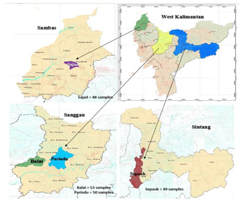
Indonesian rubber farming has the largest area in the world, but its implementation faces various risks that decrease productivity and farm income. This study is designed to specify the risk perception, risk attitude and determinant factors for smallholder rubber farmers. The research location was in four subdistricts in West Kalimantan Province, with a sample size of 200 farmers. Data collection was carried out by interview using a structured questionnaire. The risk matrix, Holt and Laury's method and the logit model were used to identify risk perception, risk attitude and determinant factors. The study results showed that most rubber farmers were risk-averse and perceived climate change, plant diseases and price change as high risks. The logit model found that farmers' age, education, rubber plantation size, rubber age, distance and use of rubber clones had a positive and significant effect on farmers' risk perception, while the family size and farming experience had a negative effect. Regarding risk attitude, the logit model found that rubber age, distance and risk perception of price change had a positive and significant effect on farmers' risk aversion, while farmers' age and use of rubber clones had a negative effect. This study recommends providing informal education to the farmers through training and counseling, encouraging the farmers to replant old or damaged rubber trees and adopt rubber clones. Furthermore, it is also necessary to improve road facilities and infrastructure, communication and transportation access to facilitate farming activities.
Citation: Imelda, Jangkung Handoyo Mulyo, Any Suryantini, Masyhuri. Understanding farmers' risk perception and attitude: A case study of rubber farming in West Kalimantan, Indonesia[J]. AIMS Agriculture and Food, 2023, 8(1): 164-186. doi: 10.3934/agrfood.2023009
Indonesian rubber farming has the largest area in the world, but its implementation faces various risks that decrease productivity and farm income. This study is designed to specify the risk perception, risk attitude and determinant factors for smallholder rubber farmers. The research location was in four subdistricts in West Kalimantan Province, with a sample size of 200 farmers. Data collection was carried out by interview using a structured questionnaire. The risk matrix, Holt and Laury's method and the logit model were used to identify risk perception, risk attitude and determinant factors. The study results showed that most rubber farmers were risk-averse and perceived climate change, plant diseases and price change as high risks. The logit model found that farmers' age, education, rubber plantation size, rubber age, distance and use of rubber clones had a positive and significant effect on farmers' risk perception, while the family size and farming experience had a negative effect. Regarding risk attitude, the logit model found that rubber age, distance and risk perception of price change had a positive and significant effect on farmers' risk aversion, while farmers' age and use of rubber clones had a negative effect. This study recommends providing informal education to the farmers through training and counseling, encouraging the farmers to replant old or damaged rubber trees and adopt rubber clones. Furthermore, it is also necessary to improve road facilities and infrastructure, communication and transportation access to facilitate farming activities.

| [1] |
Adnan KMM, Ying L, Sarker SA, et al. (2020) Simultaneous adoption of risk management strategies to manage the catastrophic risk of maize farmers in Bangladesh. GeoJournal 86: 1981–1998. https://doi.org/10.1007/s10708-020-10154-y doi: 10.1007/s10708-020-10154-y

|
| [2] |
Fahad S, Wang J, Khan AA, et al. (2018) Evaluation of farmers' attitude and perception toward production risk: Lessons from Khyber Pakhtunkhwa Province, Pakistan. Hum Ecol Risk Assess 24: 1710–1722. https://doi.org/10.1080/10807039.2018.1460799 doi: 10.1080/10807039.2018.1460799
|
| [3] |
Oyetunde-Usman Z, Olagunju KO, Ogunpaimo OR (2021) Determinants of adoption of multiple sustainable agricultural practices among smallholder farmers in Nigeria. Int Soil Water Conserv Res 9: 241–248. https://doi.org/10.1016/j.iswcr.2020.10.007 doi: 10.1016/j.iswcr.2020.10.007
|
| [4] |
Fahad S, Wang J (2018) Farmers' risk perception, vulnerability, and adaptation to climate change in rural Pakistan. Land Use Policy 79: 301–309. https://doi.org/10.1016/j.landusepol.2018.08.018 doi: 10.1016/j.landusepol.2018.08.018
|
| [5] |
Komarek AM, De Pinto A, Smith VH (2020) A review of types of risks in agriculture: What we know and what we need to know. Agric Syst 178: 102738–102747. https://doi.org/10.1016/j.agsy.2019.102738 doi: 10.1016/j.agsy.2019.102738
|
| [6] | Hardaker JB, Lien G, Anderson JR, et al. (2004) Coping with risk in agriculture, CAB International. https://doi.org/10.1079/9780851998312.0000 |
| [7] | The World Bank (2016) Agricultural Sector Risk Assessment : Methodological Guidance For Practitioners, Washington DC, World Bank Group. |
| [8] |
Tudor K, Spaulding A, Roy KD, et al. (2014) An analysis of risk management tools utilized by Illinois farmers. Agric Financ Rev 74: 69–86. https://doi.org/10.1108/AFR-09-2012-0044 doi: 10.1108/AFR-09-2012-0044
|
| [9] |
Jankelova N, Masar D, Moricova S (2017) Risk factors in the agriculture sector. Agric Econ (Czech Republic) 63: 247–258. https://doi.org/10.17221/212/2016-AGRICECON doi: 10.17221/212/2016-AGRICECON
|
| [10] |
Gebreegziabher K, Tadesse T (2014) Risk perception and management in smallholder dairy farming in Tigray, Northern Ethiopia. J Risk Res 17: 367–381. https://doi.org/10.1080/13669877.2013.815648 doi: 10.1080/13669877.2013.815648
|
| [11] |
Akhtar S, LI G cheng, Ullah R, et al. (2018) Factors influencing hybrid maize farmers' risk attitudes and their perceptions in Punjab Province, Pakistan. J Integr Agric 17: 1454–1462. https://doi.org/10.1016/S2095-3119(17)61796-9 doi: 10.1016/S2095-3119(17)61796-9
|
| [12] |
Lebel L, Lebel P (2018) Emotions, attitudes, and appraisal in the management of climate-related risks by fish farmers in Northern Thailand. J Risk Res 21: 933–951. https://doi.org/10.1080/13669877.2016.1264450 doi: 10.1080/13669877.2016.1264450
|
| [13] |
Mgale YJ, Yunxian Y (2021) Price risk perceptions and adoption of management strategies by smallholder rice farmers in Mbeya region, Tanzania. Cogent Food Agric 7: 1919370. https://doi.org/10.1080/23311932.2021.1919370 doi: 10.1080/23311932.2021.1919370
|
| [14] |
Ahmad D, Afzal M, Rauf A (2020) Environmental risks among rice farmers and factors influencing their risk perceptions and attitudes in Punjab, Pakistan. Environ Sci Pollut Res 27: 21953–21964. https://doi.org/10.1007/s11356-020-08771-8 doi: 10.1007/s11356-020-08771-8
|
| [15] |
Iqbal MA, Ping Q, Abid M, et al. (2016) Assessing risk perceptions and attitude among cotton farmers: A case of Punjab province, Pakistan. Int J Disaster Risk Reduct 16: 68–74. https://doi.org/10.1016/j.ijdrr.2016.01.009 doi: 10.1016/j.ijdrr.2016.01.009
|
| [16] |
Saqib SE, Ahmad MM, Panezai S, et al. (2016) An empirical assessment of farmers' risk attitudes in flood-prone areas of Pakistan. Int J Disaster Risk Reduct 18: 107–114. https://doi.org/10.1016/j.ijdrr.2016.06.007 doi: 10.1016/j.ijdrr.2016.06.007
|
| [17] |
Khan I, Lei H, Shah IA, et al. (2020) Farm households' risk perception, attitude and adaptation strategies in dealing with climate change: Promise and perils from rural Pakistan. Land Use Policy 91: 1–11. https://doi.org/10.1016/j.landusepol.2019.104395 doi: 10.1016/j.landusepol.2019.104395
|
| [18] |
Huet EK, Adam M, Giller KE, et al. (2020) Diversity in perception and management of farming risks in southern Mali. Agric Syst 184: 1–15. https://doi.org/10.1016/j.agsy.2020.102905 doi: 10.1016/j.agsy.2020.102905
|
| [19] |
De Salvo M, Capitello R, Gaudenzi B, et al. (2019) Risk management strategies and residual risk perception in the wine industry: A spatial analysis in Northeast Italy. Land Use Policy 83: 47–62. https://doi.org/10.1016/j.landusepol.2019.01.022 doi: 10.1016/j.landusepol.2019.01.022
|
| [20] | Sjöberg L, Moen EB, Rundmo T (2004) Explaining risk perception. An evaluation of the psychometric paradigm in risk, Rotunde. |
| [21] |
Begho T, Daubry TP, Ebuka IA (2022) What do we know about Nigerian farmers' attitudes to uncertainty and risk? A systematic review of the evidence. Sci Afr 17: e01309. https://doi.org/10.1016/j.sciaf.2022.e01309 doi: 10.1016/j.sciaf.2022.e01309
|
| [22] | Directorate General of Estate Crops (2022) Statistic of National Leading Estate Crops Comodity 2020–2022, Jakarta, Directorate General of Estate Crops, Ministry of Agriculture. |
| [23] | Sdoodee S, Rongsawat S (2012) Impact of Climate Change on Smallholders ' Rubber Production in Songkhla Province, Southern Thailand. Proceeeding of The 2012 International and National Conference For The Sustainable Community Development of "Local Community : The Foundation of Development in the ASEAN Economic Community (AEC), 81–86. |
| [24] |
Hazir MHM, Kadir RA, Gloor E, et al. (2020) Effect of agroclimatic variability on land suitability for cultivating rubber (Hevea brasiliensis) and growth performance assessment in the tropical rainforest climate of Peninsular Malaysia. Clim Risk Manag 27: 100203–100221. https://doi.org/10.1016/j.crm.2019.100203 doi: 10.1016/j.crm.2019.100203
|
| [25] |
Ali MF, Aziz AA, Sulong SH (2020) The role of decision support systems in smallholder rubber production: Applications, limitations and future directions. Comput Electron Agric 173: 105442. https://doi.org/10.1016/j.compag.2020.105442 doi: 10.1016/j.compag.2020.105442
|
| [26] |
Abdulla I, Arshad FM (2017) Exploring relationships between rubber productivity and R & D in Malaysia. Outlook Agric 46: 28–35. https://doi.org/10.1177/0030727016689731 doi: 10.1177/0030727016689731
|
| [27] |
Qi D, Zhu J, Huang Y, et al. (2021) Factors affecting technology choice behaviour of rubber smallholders: a case study in central Hainan, China. J Rubber Res 1–11. https://doi.org/10.1007/s42464-021-00096-6 doi: 10.1007/s42464-021-00096-6
|
| [28] |
Min S, Waibel H, Cadisch G, et al. (2017) The economics of smallholder rubber farming in a mountainous region of Southwest China: Elevation, ethnicity, and risk. Mt Res Dev 37: 281–293. https://doi.org/10.1659/MRD-JOURNAL-D-16-00088.1 doi: 10.1659/MRD-JOURNAL-D-16-00088.1
|
| [29] |
Jin S, Huang J, Waibel H (2020) Location and economic resilience in rubber farming communities in southwest China. China Agric Econ Rev 13: 367–396. https://doi.org/10.1108/CAER-06-2020-0153 doi: 10.1108/CAER-06-2020-0153
|
| [30] |
Goh HH, Tan KL, Khor CY, et al. (2016) Volatility and market risk of rubber price in Malaysia: Pre- and post-global financial crisis. J Quant Econ 14: 323–344. https://doi.org/10.1007/s40953-016-0037-4 doi: 10.1007/s40953-016-0037-4
|
| [31] |
Azis M, Dermoredjo SK, Sayaka B, et al. (2021) Economic perspective of indonesian rubber on agroforestry development, E3S Web Conf 305: 02007. https://doi.org/10.1051/e3sconf/202130502007 doi: 10.1051/e3sconf/202130502007
|
| [32] |
Zaw ZN, Sdoodee S, Lacote R (2017) Performances of low frequency rubber tapping system with rainguard in high rainfall area in Myanmar. Aust J Crop Sci 11: 1451–1456. https://doi.org/10.21475/ajcs.17.11.11.pne593 doi: 10.21475/ajcs.17.11.11.pne593
|
| [33] | Ismail T, Gohet E (2020) Impact of climate change on latex harvesting, Natural rubber systems and climate change (FTA Working Report), 16–18. |
| [34] |
Rivano F, Maldonado L, Simbaña B, et al. (2015) Suitable rubber growing in Ecuador: An approach to South American leaf blight. Ind Crops Prod 66: 262–270. https://doi.org/10.1016/j.indcrop.2014.12.034 doi: 10.1016/j.indcrop.2014.12.034
|
| [35] |
Olaniyi ON, Szulczyk KR (2022) Estimating the economic impact of the white root rot disease on the Malaysian rubber plantations. For Policy Econ 138: 102707. https://doi.org/10.1016/j.forpol.2022.102707 doi: 10.1016/j.forpol.2022.102707
|
| [36] |
Febbiyanti TR, Fairuza Z (2019) Identification of causes of rubber leaves outbreak in Indonesia. Indones J Nat Rubber Res 37: 193–206. https://doi.org/10.22302/ppk.jpk.v37i2.616 doi: 10.22302/ppk.jpk.v37i2.616
|
| [37] |
Jin S, Min S, Huang J, et al. (2021) Falling price induced diversification strategies and rural inequality: Evidence of smallholder rubber farmers. World Dev 146: 105604. https://doi.org/10.1016/j.worlddev.2021.105604 doi: 10.1016/j.worlddev.2021.105604
|
| [38] |
Nicod T, Bathfield B, Bosc PM, et al. (2020) Households' livelihood strategies facing market uncertainties: How did Thai farmers adapt to a rubber price drop? Agric Syst 182: 1–11. https://doi.org/10.1016/j.agsy.2020.102846 doi: 10.1016/j.agsy.2020.102846
|
| [39] | Penot E, Chambon B, Wibawa G (2017) An history of Rubber Agroforestry Systems development in Indonesia and Thailand as alternatives for a sustainable agriculture and income stability, IRRDB International Rubber Conference, Bali. |
| [40] |
Penot E, Thériez M, Michel I, et al. (2022) Agroforestry rubber networks and farmers groups in Phatthalung area in Southern Thailand: A potential for an innovation platform? For Soc 6: 503–526. https://doi.org/10.24259/fs.v6i2.12481 doi: 10.24259/fs.v6i2.12481
|
| [41] |
Ali MF, Akber MA, Smith C, et al. (2021) The dynamics of rubber production in Malaysia: Potential impacts, challenges and proposed interventions. For Policy Econ 127: 102449. https://doi.org/10.1016/j.forpol.2021.102449 doi: 10.1016/j.forpol.2021.102449
|
| [42] |
Andriesse E, Tanwattana P (2018) Coping with the end of the commodities boom: Rubber smallholders in Southern Thailand oscillating between near-poverty and middle-class status. J Dev Soc 34: 77–102. https://doi.org/10.1177/0169796X17752420 doi: 10.1177/0169796X17752420
|
| [43] |
Khan NA, Gao Q, Iqbal MA, et al. (2020) Modeling food growers ' perceptions and behavior towards environmental changes and its induced risks : evidence from Pakistan. Environ Sci Pollut Res 27: 20292–20308. https://doi.org/10.1007/s11356-020-08341-y doi: 10.1007/s11356-020-08341-y
|
| [44] |
Ahmad D, Afzal M, Rauf A (2019) Analysis of wheat farmers' risk perceptions and attitudes : evidence from Punjab, Pakistan. Nat Hazards 95: 845–861. https://doi.org/10.1007/s11069-018-3523-5 doi: 10.1007/s11069-018-3523-5
|
| [45] |
Lebel P, Whangchai N, Chitmanat C, et al. (2015) Climate risk management in river-based tilapia cage culture in northern Thailand. Int J Clim Chang Strateg Manag 7: 476–498. https://doi.org/10.1108/IJCCSM-01-2014-0018 doi: 10.1108/IJCCSM-01-2014-0018
|
| [46] |
Alam A, Guttormsen AG (2019) Risk in aquaculture : Farmers' perceptions and management strategies in Bangladesh. Aquac Econ Manag 23: 359–381. https://doi.org/10.1080/13657305.2019.1641568 doi: 10.1080/13657305.2019.1641568
|
| [47] |
Meraner M, Finger R (2017) Risk perceptions, preferences and management strategies: Evidence from a case study using German livestock farmers. J Risk Res 22: 110–135. https://doi.org/10.1080/13669877.2017.1351476 doi: 10.1080/13669877.2017.1351476
|
| [48] |
Bishu KG, O'Reilly S, Lahiff E, et al. (2016) Cattle farmers' perceptions of risk and risk management strategies: Evidence from Northern Ethiopia. J Risk Res 21: 579–598. https://doi.org/10.1080/13669877.2016.1223163 doi: 10.1080/13669877.2016.1223163
|
| [49] | Thomas G (2018) Risk Management in Agriculture, Scotlandia, The Scottish Parliament. |
| [50] |
Durrani H, Syed A, Khan A, et al. (2021) Understanding farmers' risk perception to drought vulnerability in Balochistan, Pakistan. AIMS Agric Food 6: 82–105. https://doi.org/10.3934/agrfood.2021006 doi: 10.3934/agrfood.2021006
|
| [51] |
Yarong L, Minpeng C (2021) Farmers' perception on combined climatic and market risks and their adaptive behaviors : a case in Shandong Province. Environ Dev Sustain 23: 13042–13061. https://doi.org/10.1007/s10668-020-01198-8 doi: 10.1007/s10668-020-01198-8
|
| [52] |
Onyeneke RU, Nwajiuba CA, Emenekwe CC, et al. (2019) Climate change adaptation in Nigerian agricultural sector: A systematic review and resilience check of adaptation measures. AIMS Agric Food 4: 967–1006. https://doi.org/10.3934/agrfood.2019.4.967 doi: 10.3934/agrfood.2019.4.967
|
| [53] |
He R, Jin J, Kuang F, et al. (2020) Farmers' risk cognition, risk preferences and climate change adaptive behavior: A structural equation modeling approach. Int J Environ Res Public Health 17: 85–97. https://doi.org/10.3390/ijerph17010085 doi: 10.3390/ijerph17010085
|
| [54] |
Huong NTL, Bo YS, Fahad S (2017) Farmers' perception, awareness and adaptation to climate change: evidence from northwest Vietnam. Int J Clim Chang Strateg Manag 9: 555–576. https://doi.org/10.1108/IJCCSM-02-2017-0032 doi: 10.1108/IJCCSM-02-2017-0032
|
| [55] |
Iqbal MA, Ping Q, Zafar MU, et al. (2018) Farm risk sources and their mitigation: A case of cotton growers in Punjab. Pakistan J Agric Sci 55: 683–690. https://doi.org/10.21162/PAKJAS/18.7070 doi: 10.21162/PAKJAS/18.7070
|
| [56] |
Le TC, Cheong F (2010) Perceptions of risk and risk management in vietnamese catfish farming: An empirical study. Aquac Econ Manag 14: 282–314. https://doi.org/10.1080/13657305.2010.526019 doi: 10.1080/13657305.2010.526019
|
| [57] | Hillson D, Murray-webster R (2005) Understanding and Managing Risk Attitude, United States of America. |
| [58] | Pindyck RS, Rubinfeld DL (2013) Microeconomics, United States of America, Pearson. |
| [59] | Theuvsen L (2013) Risks and Risk Management in Agriculture. |
| [60] | Directorate General of Estate Crops (2019) Tree Crop Estate Statistics of Indonesia (Rubber) 2018–2020, Jakarta, Directorate General of Estates Crops Ministry of Agriculture. |
| [61] |
Winarni B, Lahjie AM, Simarangkir BDAS, et al. (2017) Forest gardens management under traditional ecological knowledge in West Kalimantan, Indonesia. Biodiversitas 19: 77–84. https://doi.org/10.13057/biodiv/d190113 doi: 10.13057/biodiv/d190113
|
| [62] | Statistics of Kalimantan Barat Province (2022) Kalimantan Barat Province in Figures 2022, Pontianak, Statistics of Kalimantan Barat Province. |
| [63] | Moser S, Mußhoff O (2017) Comparing the use of risk-influencing production inputs and experimentally measured risk attitude: Do the decisions of indonesian small-scale rubber farmers match? Ger J Agric Econ 66: 124–139. |
| [64] |
Holt CA, Laury SK (2002) Risk aversion and incentive effects. Am Econ Rev 92: 1644–1655. https://doi.org/10.1257/000282802762024700 doi: 10.1257/000282802762024700
|
| [65] |
Michailova J, Mačiulis A, Tvaronavičienė M (2017) Overconfidence, risk aversion and individual financial decisions in experimental asset markets. Econ Res 30: 1119–1131. https://doi.org/10.1080/1331677X.2017.1311234 doi: 10.1080/1331677X.2017.1311234
|
| [66] | Hosmer DW, Lemeshow S, Sturdivant RX (2013) Applied Logistic Regression., United States of America, Wiley. https://doi.org/10.1002/9781118548387 |
| [67] | Pedace R (2013) Econometrics For Dummies, United States of America, John Wiley & Sons Inc. |
| [68] | Glorya MJ, Nugraha A (2019) Private Sector Initiatives To Boost Productivity of Cocoa, Coffee, and Rubber in Indonesia, Jakarta. https://doi.org/10.35497/291601 |
| [69] | Ruangsri K, Makkaew K, Sdoodee S (2015) The impact of rainfall fluctuation on days and rubber productivity in Songkhla Province. Int J Agric Technol 11: 181–191. |
| [70] |
Thaochan N, Pornsuriya C, Chairin T, et al. (2020) Roles of systemic fungicide in antifungal activity and induced defense responses in rubber tree (Hevea brasiliensis) against leaf fall disease caused by Neopestalotiopsis cubana. Physiol Mol Plant Pathol 111: 101511. https://doi.org/10.1016/j.pmpp.2020.101511 doi: 10.1016/j.pmpp.2020.101511
|
| [71] |
Go WZ, Chin KL, H'ng PS, et al. (2021) Virulence of rigidoporus microporus isolates causing white root rot disease on rubber trees (Hevea brasiliensis) in Malaysia. Plants 10: 2123. https://doi.org/10.3390/plants10102123 doi: 10.3390/plants10102123
|
| [72] |
Siri-udom S, Suwannarach N, Lumyong S (2017) Applications of volatile compounds acquired from Muscodor heveae against white root rot disease in rubber trees (Hevea brasiliensis Müll. Arg.) and relevant allelopathy effects. Fungal Biol 121: 573–581. https://doi.org/10.1016/j.funbio.2017.03.004 doi: 10.1016/j.funbio.2017.03.004
|
| [73] |
Syahza A, Backe D, Asmit B (2018) Natural rubber institutional arrangement in efforts to accelerate rural economic development in the province of Riau. Int J Law Manag 60: 1509–1521. https://doi.org/10.1108/IJLMA-10-2017-0257 doi: 10.1108/IJLMA-10-2017-0257
|
| [74] | Syarifa LF, Agustina DS, Nancy C, et al. (2016) Low Rubber Prices Impact on Socio Economic Condition of Rubber Smallholders in South Sumatera. Indones J Nat Rubber Res 34: 119–126. |
| [75] |
Ullah R, Shivakoti GP, Ali G (2015) Factors effecting farmers' risk attitude and risk perceptions: The case of Khyber Pakhtunkhwa, Pakistan. Int J Disaster Risk Reduct 13: 151–157. https://doi.org/10.1016/j.ijdrr.2015.05.005 doi: 10.1016/j.ijdrr.2015.05.005
|
| [76] |
Islam MD Il, Rahman A, Sarker MNI, et al. (2021) Factors influencing rice farmers' risk attitudes and perceptions in bangladesh amid environmental and climatic issues. Polish J Environ Stud 30: 177–187. https://doi.org/10.15244/pjoes/120365 doi: 10.15244/pjoes/120365
|
| [77] |
Sun Y, Han Z (2018) Climate change risk perception in Taiwan: Correlation with individual and societal factors. Int J Environ Res Public Health 15: 91. https://doi.org/10.3390/ijerph15010091 doi: 10.3390/ijerph15010091
|
| [78] |
Rizwan M, Ping Q, Saboor A, et al. (2020) Measuring rice farmers' risk perceptions and attitude: Evidence from Pakistan. Hum Ecol Risk Assess 26: 1832–1847. https://doi.org/10.1080/10807039.2019.1602753 doi: 10.1080/10807039.2019.1602753
|
| [79] |
Fauzi IR, Syarifa LF, Herlinawati E, et al. (2014) Performance of tapping premium system in some rubber plantation enterprises. Indones J Nat Rubber Res 32: 157–180. https://doi.org/10.22302/ppk.jpk.v32i2.162 doi: 10.22302/ppk.jpk.v32i2.162
|
| [80] | Oduro-ofori E, Aboagye Anokye P, Acquaye NEA (2014) Effects of education on the agricultural productivity of farmers in offinso municipality. Int J Dev Res 4: 1951–1960. |
| [81] |
Paltasingh KR, Goyari P (2018) Impact of farmer education on farm productivity under varying technologies: case of paddy growers in India. Agric Food Econ 6: 7. https://doi.org/10.1186/s40100-018-0101-9 doi: 10.1186/s40100-018-0101-9
|
| [82] |
Asadullah MN, Rahman S (2009) Farm productivity and efficiency in rural Bangladesh: The role of education revisited. Appl Econ 41: 17–33. https://doi.org/10.1080/00036840601019125 doi: 10.1080/00036840601019125
|
| [83] |
Tongkaemkaew U, Chambon B (2018) Rubber plantation labor and labor movements as rubber prices decrease in Southern Thailand. For Soc 2: 18–27. https://doi.org/10.24259/fs.v2i1.3641 doi: 10.24259/fs.v2i1.3641
|
| [84] | Tanakasempipat P (2019) Reuters, Top rubber producer Thailand hit by fungal disease outbreak. Available from: https://www.reuters.com/article/us-thailand-rubber-idUSKBN1X0118. |
| [85] |
Razar RM, Hamid NRA, Ghani ZA (2021) GxE effect and stability analyses of selected rubber clones (Hevea brasiliensis) in Malaysia. J Rubber Res 24: 475–487. https://doi.org/10.1007/s42464-021-00115-6 doi: 10.1007/s42464-021-00115-6
|
| [86] |
Ouattara PD, Kouassi E, Egbendéwé AYG, et al. (2019) Risk aversion and land allocation between annual and perennial crops in semisubsistence farming: a stochastic optimization approach. Agric Econ (United Kingdom) 50: 329–339. https://doi.org/10.1111/agec.12487 doi: 10.1111/agec.12487
|
| [87] |
Djanibekov U, Villamor GB (2017) Market-based instruments for risk-averse farmers: Rubber agroforest conservation in Jambi Province, Indonesia. Environ Dev Econ 22: 133–155. https://doi.org/10.1017/S1355770X16000310 doi: 10.1017/S1355770X16000310
|
| [88] |
Sitepu MH, McKay A, Holt RJ (2019) An approach for the formulation of sustainable replanting policies in the Indonesian natural rubber industry. J Clean Prod 241: 118357–118368. https://doi.org/10.1016/j.jclepro.2019.118357 doi: 10.1016/j.jclepro.2019.118357
|
| [89] |
Penot E, Ilahang (2021) Rubber Agroforestry Systems (RAS) in West Kalimantan, Indonesia: An historical perspective. E3S Web Conf 305: 02001. https://doi.org/10.1051/e3sconf/202130502001 doi: 10.1051/e3sconf/202130502001
|


Figures(5) / Tables(5)

Imelda, Jangkung Handoyo Mulyo, Any Suryantini, Masyhuri. Understanding farmers' risk perception and attitude: A case study of rubber farming in West Kalimantan, Indonesia[J]. AIMS Agriculture and Food, 2023, 8(1): 164-186. doi: 10.3934/agrfood.2023009


 DownLoad: