Estimating the volume of food plays an important role in diet monitoring. However, it is difficult to perform this estimation automatically and accurately. A new method based on the multi-layer superpixel technique is proposed in this paper to avoid tedious human-computer interaction and improve estimation accuracy. Our method includes the following steps: 1) obtain a pair of food images along with the depth information using a stereo camera; 2) reconstruct the plate plane from the disparity map; 3) warp the input image and the disparity map to form a new direction of view parallel to the plate plane; 4) cut the warped image into a series of slices according to the depth information and estimate the occluded part of the food; and 5) rescale superpixels for each slice and estimate the food volume by accumulating all available slices in the segmented food region. Through a combination of image data and disparity map, the influences of noise and visual error in existing interactive food volume estimation methods are reduced, and the estimation accuracy is improved. Our experiments show that our method is effective, accurate and convenient, providing a new tool for promoting a balanced diet and maintaining health.
Citation: Xin Zheng, Chenhan Liu, Yifei Gong, Qian Yin, Wenyan Jia, Mingui Sun. Food volume estimation by multi-layer superpixel[J]. Mathematical Biosciences and Engineering, 2023, 20(4): 6294-6311. doi: 10.3934/mbe.2023271
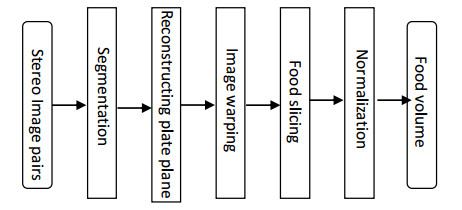
Estimating the volume of food plays an important role in diet monitoring. However, it is difficult to perform this estimation automatically and accurately. A new method based on the multi-layer superpixel technique is proposed in this paper to avoid tedious human-computer interaction and improve estimation accuracy. Our method includes the following steps: 1) obtain a pair of food images along with the depth information using a stereo camera; 2) reconstruct the plate plane from the disparity map; 3) warp the input image and the disparity map to form a new direction of view parallel to the plate plane; 4) cut the warped image into a series of slices according to the depth information and estimate the occluded part of the food; and 5) rescale superpixels for each slice and estimate the food volume by accumulating all available slices in the segmented food region. Through a combination of image data and disparity map, the influences of noise and visual error in existing interactive food volume estimation methods are reduced, and the estimation accuracy is improved. Our experiments show that our method is effective, accurate and convenient, providing a new tool for promoting a balanced diet and maintaining health.

| [1] | World Health Organisation, Obesity and overweight, 2018. Available from: http://www.who.int/mediacentre/factsheets/fs311/en/. |
| [2] | G. Ni, J. Zhang, F. Zheng, The current situation and trend of obesity epidemic in China, Food Nutr. China, 19 (2013), 70–74. |
| [3] | World Health Organisation, What are the health consequences of being overweight?, 2013. Available from: https://www.who.int/features/qa/49/en/. |
| [4] |
F. Lo, Y. Sun, J. Qiu, B. Lo, Image-based food classification and volume estimation for dietary assessment: A review, IEEE J. Biomed. Health Inform., 24 (2020), 1926–1939. https://doi.org/10.1109/JBHI.2020.2987943 doi: 10.1109/JBHI.2020.2987943

|
| [5] |
W. Tay, B. Kaur, R. Quek, Current developments in digital quantitative volume estimation for the optimisation of dietary assessment, Nutrients, 12 (2020), 1167. https://doi.org/10.3390/nu12041167 doi: 10.3390/nu12041167
|
| [6] |
I. Nyalala, C. Okinda, K. Chen, T. Korohou, L. Nyalala, C. Qi, Weight and volume estimation of poultry and products based on computer vision systems: A review, Poult. Sci., 100 (2021). https://doi.org/10.1016/j.psj.2021.101072 doi: 10.1016/j.psj.2021.101072
|
| [7] |
V. B. Raju, E. Sazonov, A Systematic Review of Sensor-Based Methodologies for Food Portion Size Estimation, IEEE Sens. J., 21 (2021), 12882–12899. https://doi.org/10.1109/JSEN.2020.3041023 doi: 10.1109/JSEN.2020.3041023
|
| [8] |
M. Sun, Q. Liu, K. Schmidt, J. Yang, N. Yao, J. Fernstrom, et al., Determination of food portion size by image processing, Proc. Annu. Int. Conf. IEEE Eng. Med. Biol. Soc., (2008), 871–874. https://doi.org/10.1109/EMBS10205.2008 doi: 10.1109/EMBS10205.2008
|
| [9] |
Y. Yang, W. Jia, T. Bucher, H. Zhang, M. Sun, Image-based food portion size estimation using a smartphone without a fiducial marker, Public Health Nutrition, 22 (2018), 1180–1192. https://doi.org/10.1017/S136898001800054X doi: 10.1017/S136898001800054X
|
| [10] |
F. Zhu, M. Bosch, I. Woo, S. Kim, C. Boushey, D. Ebert, et al., The use of mobile devices in aiding dietary assessment and evaluation, IEEE J. Sel. Top. Sign. Proces., 4 (2010), 756–766. https://doi.org/10.1109/JSTSP.2010.2051471 doi: 10.1109/JSTSP.2010.2051471
|
| [11] |
H. C. Chen, Y. Yue, Z. Li, J. Fernstrom, Y. Bai, C. Li, et al., Accuracy of food portion size estimation from digital pictures acquired by a chest-worn camera, Public Health Nutr., 17 (2014), 1671–1681. https://doi.org/10.1017/S1368980013003236 doi: 10.1017/S1368980013003236
|
| [12] |
H. Chen, W. Jia, Y. Yue, Z. Li, Y. Sun, J. Fernstrom, et al., Model-based measurement of food portion size for image-based dietary assessment using 3D/2D registration, Meas. Sci. Technol., 24 (2013). https://doi.org/10.1088/0957-0233/24/10/105701 doi: 10.1088/0957-0233/24/10/105701
|
| [13] |
C. Xu, Y. He, N. Khanna, C. Boushey, E. Delp, Model-based food volume estimation using 3D pose, IEEE Int. Conf. Image Process., (2013), 2534–2538. https://doi.org/10.1109/ICIP.2013.6738522 doi: 10.1109/ICIP.2013.6738522
|
| [14] |
J. Dehais, M. Anthimopoulos, S. Shevchik, S. Mougiakakou, Two-view 3D reconstruction for food volume estimation, IEEE Trans Multimedia, 19 (2017), 1090–1099. https://doi.org/10.1109/TMM.2016.2642792 doi: 10.1109/TMM.2016.2642792
|
| [15] |
M. Puri, Z. Zhu, Q. Yu, A. Divakaran, H. Sawhney, Recognition and volume estimation of food intake using a mobile device, Workshop Appl. Comput. Vis., (2009), 1–8. https://doi.org/10.1109/WACV.2009.5403087 doi: 10.1109/WACV.2009.5403087
|
| [16] |
M. Rahman, Q. Li, M. Pickering, M. Frater, D. Kerr, C. Bouchey, et al., Food volume estimation in a mobile phone based dietary assessment system, Int. Conf. Signal Image Technol. Internet Based Syst., (2012), 988–995. https://doi.org/10.1109/SITIS.2012.146 doi: 10.1109/SITIS.2012.146
|
| [17] |
T. Suzuki, K. Futatsuishi, K. Yokoyama, N. Amaki, Point cloud processing method for food volume estimation based on dish space, Proc. Annu. Int. Conf. IEEE Eng. Med. Biol. Soc., (2020), 5665–5668. https://doi.org/10.1109/EMBC44109.2020.9175807 doi: 10.1109/EMBC44109.2020.9175807
|
| [18] | H. Yin, 3D reconstruction from infrared stereo image pairs, Masters Abstr. Inte., 2013. |
| [19] |
L. Zhou, C. Zhang, F. Liu, Z. Qiu, Y. He, Application of deep learning in food: A review. Compr. Rev. Food Sci. Food Saf., 18 (2019), 1793–1811. https://doi.org/10.1111/1541-4337.12492 doi: 10.1111/1541-4337.12492
|
| [20] |
F. Lo, Y. Sun, J. Qiu, B. Lo, Food volume estimation based on deep learning view synthesis from a single depth map, Nutr., 10 (2018). https://doi.org/10.3390/nu10122005 doi: 10.3390/nu10122005
|
| [21] |
F. Boemer, E. Ratner, A. Lendasse, Parameter-free image segmentation with SLIC, Neurocomputing, 277 (2018), 228–236. https://doi.org/10.1016/j.neucom.2017.05.096 doi: 10.1016/j.neucom.2017.05.096
|
| [22] |
J. Hou, C. Sha, L. Chi, Q. Xia, N. Qi, Merging dominant sets and DBSCAN for robust clustering and image segmentation, IEEE Int. Conf. Image Process., (2014), 4422–4426. https://doi.org/10.1109/ICIP.2014.7025897 doi: 10.1109/ICIP.2014.7025897
|
| [23] |
P. Torr, A. Zisserman, MLESAC: A New Robust Estimator with Application to Estimating Image Geometry, Comput. Vis. Image Und., 78 (2000), 138–156, https://doi.org/10.1006/cviu.1999.0832 doi: 10.1006/cviu.1999.0832
|


Figures(13) / Tables(3)

Xin Zheng, Chenhan Liu, Yifei Gong, Qian Yin, Wenyan Jia, Mingui Sun. Food volume estimation by multi-layer superpixel[J]. Mathematical Biosciences and Engineering, 2023, 20(4): 6294-6311. doi: 10.3934/mbe.2023271


 DownLoad: