This research looks into the main DNA markers and the limits of their application in molecular phylogenetic analysis. Melatonin 1B (MTNR1B) receptor genes were analyzed from various biological sources. Based on the coding sequences of this gene, using the class Mammalia as example, phylogenetic reconstructions were made to study the potential of mtnr1b as a DNA marker for phylogenetic relationships investigating. The phylogenetic trees were constructed using NJ, ME and ML methods that establish the evolutionary relationships between different groups of mammals. The resulting topologies were generally in good agreement with topologies established on the basis of morphological and archaeological data as well as with other molecular markers. The present divergences provided a unique opportunity for evolutionary analysis. These results suggest that the coding sequence of the MTNR1B gene can be used as a marker to study the relationships of lower evolutionary levels (order, species) as well as to resolve deeper branches of the phylogenetic tree at the infraclass level.
Citation: Ekaterina Y. Kasap, Оlga K. Parfenova, Roman V. Kurkin, Dmitry V. Grishin. Bioinformatic analysis of the coding region of the melatonin receptor 1b gene as a reliable DNA marker to resolve interspecific mammal phylogenetic relationships[J]. Mathematical Biosciences and Engineering, 2023, 20(3): 5430-5447. doi: 10.3934/mbe.2023251
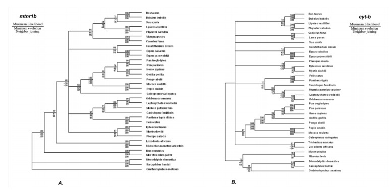
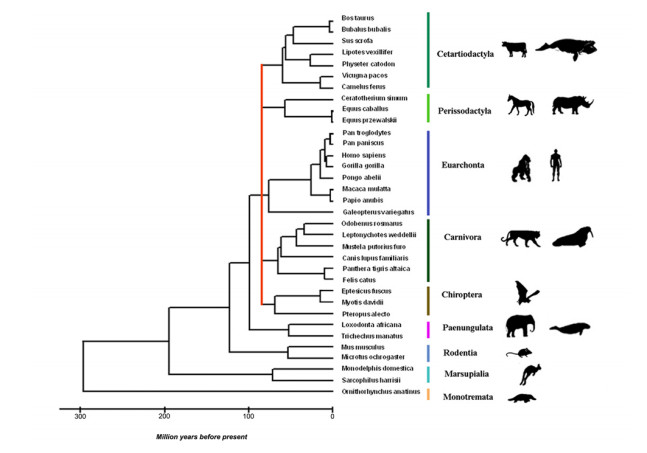
This research looks into the main DNA markers and the limits of their application in molecular phylogenetic analysis. Melatonin 1B (MTNR1B) receptor genes were analyzed from various biological sources. Based on the coding sequences of this gene, using the class Mammalia as example, phylogenetic reconstructions were made to study the potential of mtnr1b as a DNA marker for phylogenetic relationships investigating. The phylogenetic trees were constructed using NJ, ME and ML methods that establish the evolutionary relationships between different groups of mammals. The resulting topologies were generally in good agreement with topologies established on the basis of morphological and archaeological data as well as with other molecular markers. The present divergences provided a unique opportunity for evolutionary analysis. These results suggest that the coding sequence of the MTNR1B gene can be used as a marker to study the relationships of lower evolutionary levels (order, species) as well as to resolve deeper branches of the phylogenetic tree at the infraclass level.

| [1] |
V. V. Grechko, Molecular DNA markers in phylogeny and systematics, Russ. J. Genet., 38 (2002), 851–868. https://doi.org/10.1023/A:1016890509443 doi: 10.1023/A:1016890509443

|
| [2] |
A. Patwardhan, S. Ray, A. Roy, Molecular markers in phylogenetic studies—A review, J. Phylogen. Evolution Biol., 2 (2014), 1–9. https://doi.org/10.4172/2329-9002.1000131 doi: 10.4172/2329-9002.1000131
|
| [3] |
L. Wei, Selection On synonymous Mutations Revealed by 1135 Genomes of Arabidopsis thaliana, Evol. Bioinform. Online, 16 (2020) 1176934320916794. https://doi.org/10.1177/1176934320916794 doi: 10.1177/1176934320916794
|
| [4] |
W. M. Brown, M. George, A. C. Wilson, Rapid evolution of animal mitochondrial DNA, PNAS, 76 (1979), 1967–1971. https://doi.org/10.1073/pnas.76.4.1967 doi: 10.1073/pnas.76.4.1967
|
| [5] | A. A. Bannikova, Molecular markers and modern phylogenetics of mammals, Zh. Obshch. Biol., 65 (2004), 278–305. (in Russian) |
| [6] | A. C. Wilson, R. L. Cann, S. M. Carr, M. George, U. B. Gyllensten, K. M. Helm-Bychowski, et al., Mitochondrial DNA and two perspectives on evolutionary genetics, Biol. J. Linnean Soc., 26 (1985), 375–400. doi.org/10.1111/j.1095-8312.1985.tb02048.x |
| [7] |
G. Pesole, E. Sbisa, G. Preparata, C. Saccone, The evolution of the mitochondrial D-loop region and the origin of modern man, Mol. Biol. Evol., 9 (1992), 587–598. https://doi.org/10.1093/oxfordjournals.molbev.a040747 doi: 10.1093/oxfordjournals.molbev.a040747
|
| [8] | W. M. Brown, E. H. Prager, A. Wang, A. C. Wilson, Mitochondrial DNA sequences of primates: Tempo and mode of evolution, J. Mol. Evol., 18 (1982), 225–239. |
| [9] |
H. Cernohorska, S. Kubickova, O. Kopecna, A. I. Kulemzina, P. L. Perelman, F. F. Elder, et al., Molecular cytogenetic insights to the phylogenetic affinities of the giraffe (Giraffa camelopardalis) and pronghorn (Antilocapra americana), Chromosome Res., 2 (2013), 447–460. https://doi.org/10.1007/s10577-013-9361-0 doi: 10.1007/s10577-013-9361-0
|
| [10] |
D. Huchon, O. Madsen, M. Sibbald, K. Ament, M. J. Stanhope, F. Catzeflis, et al., Rodent phylogeny and a timescale for the evolution of glires: Evidence from an extensive taxon sampling using three nuclear genes, Mol. Biol. Evol., 19 (2002), 1053–1065. https://doi.org/10.1093/oxfordjournals.molbev.a004164 doi: 10.1093/oxfordjournals.molbev.a004164
|
| [11] | M. Weksler, Phylogeny of Neotropical oryzomyine rodents (Muridae: Sigmodontinae) based on the nuclear IRBP exon, Mol. Phylogenet. Evol., 29 (2003), 331–349. doi.org/10.1016/S1055-7903(03)00132-5 |
| [12] |
E. Zietkiewicz, A. Rafalski, D. Labuda, Genome fingerprinting by simple sequence repeat (SSR)-anchored polymerase chain reaction amplification, Genomics, 20 (1994), 176–183. https://doi.org/10.1006/geno.1994.1151 doi: 10.1006/geno.1994.1151
|
| [13] |
H. Nybom, Comparison of different nuclear DNA markers for estimating intraspecific genetic diversity in plants, Mol Ecol., 13 (2004), 1143–1155. https://doi.org/10.1111/j.1365-294X.2004.02141.x doi: 10.1111/j.1365-294X.2004.02141.x
|
| [14] |
S. R. Pandi-Perumal, V. Srinivasan, G. J. Maestroni, D. P. Cardinali, B. Poeggeler, R. Hardeland, Melatonin: Nature's most versatile biological signal? FEBS, 273 (2006), 2813–2838. https://doi.org/10.1111/j.1742-4658.2006.05322.x doi: 10.1111/j.1742-4658.2006.05322.x
|
| [15] |
A. F. Alamdari, S. Rahnemayan, H. Rajabi, N. Vahed, H. R. K. Kashani, A. Rezabakhsh, et al., Melatonin as a promising modulator of aging related neurodegenerative disorders: Role of microRNAs, Pharmacol. Res., 173 (2021), 105839. https://doi.org/10.1016/j.phrs.2021.105839 doi: 10.1016/j.phrs.2021.105839
|
| [16] | S. Arias-Santiago, J. Aneiros-Fernández, B. Arias-Santiago, M. S. Girón-Prieto, M. Caba-Molina, A. López-Valverde, et al., MTNR1A receptor expression in normal and pathological human salivary glands, Anticancer Res., 32 (2012), 4765–4771. |
| [17] |
Y. Y. Li, H. Wang, Y. Y. Zhang, Melatonin receptor 1B gene rs10830963 C/G polymorphism associated with type 2 diabetes mellitus: An updated meta-analysis of 13,752 participants, Heliyon, 8 (2022), e11786. https://doi.org/10.1016/j.heliyon.2022.e11786 doi: 10.1016/j.heliyon.2022.e11786
|
| [18] |
N. R. Sundaresan, M. D. Marcus Leo, J. Subramani, D. Anish, M. Sudhagar, K. A. Ahmed, et al., Expression analysis of melatonin receptor subtypes in the ovary of domestic chicken, Vet. Res. Commun., 33 (2009), 49–56. https://doi.org/10.1007/s11259-008-9071-9 doi: 10.1007/s11259-008-9071-9
|
| [19] |
C. Jones, G. Helfer, R. Brandstätter, Melatonin receptor expression in the zebra finch brain and peripheral tissues, Chronobiol. Int., 29 (2012), 189–202. https://doi.org/10.3109/07420528.2011.642912 doi: 10.3109/07420528.2011.642912
|
| [20] |
D. Y. Li, D. G. Smith, R. Hardeland, M. Y. Yang, H. L. Xu, L. Zhang, et al., Melatonin receptor genes in vertebrates, Int. J. Mol. Sci., 14 (2013), 11208–11223. https://doi.org/10.3390/ijms140611208 doi: 10.3390/ijms140611208
|
| [21] |
C. von Gall, J. H. Stehle, D. R. Weaver, Mammalian melatonin receptors: molecular biology and signal transduction, Cell Tissue Res., 309 (2002), 151–162. https://doi.org/10.1007/s00441-002-0581-4 doi: 10.1007/s00441-002-0581-4
|
| [22] |
M. Migaud, A. Daveau, B. Malpaux, MTNR1A melatonin receptors in the ovine premammillary hypothalamus: day-night variation in the expression of the transcripts, Biol. Reprod., 72 (2005), 393–398. https://doi.org/10.1095/biolreprod.104.030064 doi: 10.1095/biolreprod.104.030064
|
| [23] |
J. Drew, P. Barrett, J. Mercer, K. Moar, E. Canet, P. Delagrange, et al., Localization of the melatonin-related receptor in the rodent brain and peripheral tissues, J. Neuroendocrinol., 13 (2001), 453–458. https://doi.org/10.1046/j.1365-2826.2001.00651.x doi: 10.1046/j.1365-2826.2001.00651.x
|
| [24] |
L. Pinato, D. Ramos, A. Hataka, P. S. Rossignoli, M. D. J. Granado, M. C. Mazzetto, et al., Day/night expression of MT1 and MT2 receptors in hypothalamic nuclei of the primate Sapajus paella, J. Chem. Neuroanat., 81 (2017), 10–17. https://doi.org/10.1016/j.jchemneu.2017.01.005 doi: 10.1016/j.jchemneu.2017.01.005
|
| [25] |
H. Ma, J. Kang, W. Fan, H. He, F. Huang, ROR: Nuclear receptor for melatonin or not? Molecules, 26 (2021), 2693. https://doi.org/10.3390/molecules26092693 doi: 10.3390/molecules26092693
|
| [26] |
S. D. Huo, R. J. Long, Melatonin receptor (MTNR1A and MTNR2B) expression during the breeding season in the yak (Bos grunniens), Czech J. Anim. Sci., 59 (2014), 140–145. https://doi.org/10.17221/7294-CJAS doi: 10.17221/7294-CJAS
|
| [27] |
J. Baker, K. Kimpinski, Role of melatonin in blood pressure regulation: An adjunct anti-hypertensive agent, CEPP, 45 (2018), 755–766. https://doi.org/10.1111/1440-1681.12942 doi: 10.1111/1440-1681.12942
|
| [28] |
M. A. Quera-Salva, U. Kilic-Huck, M. F. Vecchierini, Members of the MEL consensus group of the SFRMS. Melatonin (MEL) and its use in circadian rhythm sleep-wake disorders: Recommendations of the French Medical and Research Sleep Society (SFRMS), Rev. Neurol. (Paris)., 177 (2021), 235–244. https://doi.org/10.1016/j.neurol.2020.07.021 doi: 10.1016/j.neurol.2020.07.021
|
| [29] |
L. A. Ostrin, Ocular and systemic melatonin and the influence of light exposure, Clin. Exp. Optom., 102 (2019), 99–108. https://doi.org/10.1111/cxo.12824 doi: 10.1111/cxo.12824
|
| [30] |
Y. Tao, B. Hu, Z. Ma, H. Li, E. Du, G. Wang, et al., Intravitreous delivery of melatonin affects the retinal neuron survival and visual signal transmission: in vivo and ex vivo study, Drug Deliv., 27 (2020), 1386–1396. https://doi.org/10.1080/10717544.2020.1818882 doi: 10.1080/10717544.2020.1818882
|
| [31] |
S. Gurunathan, M. Qasim, M. H. Kang, J. H. Kim, Role and therapeutic potential of melatonin in various type of cancers, Onco. Targets Ther., 14 (2021), 2019–2052. https://doi.org/10.2147/OTT.S298512 doi: 10.2147/OTT.S298512
|
| [32] |
Y. J. Guh, T. K. Tamai, T. Yoshimura, The underlying mechanisms of vertebrate seasonal reproduction, Proc. Jpn. Acad. Ser. B Phys. Biol. Sci., 95 (2019), 343–357. https://doi.org/10.2183/pjab.95.025 doi: 10.2183/pjab.95.025
|
| [33] |
M. V. Danilova, E. N. Usoltseva, Significance of the pineal gland hormone melatonin in maintaining the health of women of reproductive age (a review), Obstetr. Gynecol. Reproduct., 13 (2019), 337–344. https://doi.org/10.17749/2313-7347.2019.13.4.337-344 doi: 10.17749/2313-7347.2019.13.4.337-344
|
| [34] |
C. C. Maganhin, L. F. Fuchs, R. S. Simões, R. M. Oliveira-Filho, M. de Jesus Simões, E. C. Baracat, et al., Effects of melatonin on ovarian follicles, Eur. J. Obstet.Gynecol. Reprod. Biol., 166 (2013), 178–184. https://doi.org/10.1016/j.ejogrb.2012.10.006 doi: 10.1016/j.ejogrb.2012.10.006
|
| [35] |
J. S. Heo, S. Pyo, J. Y. Lim, D. W. Yoon, B. Y. Kim, J. H. Kim, et al., Biological effects of melatonin on human adipose‑derived mesenchymal stem cells, Int. J. Mol. Med., 44 (2019), 2234–2244. https://doi.org/10.3892/ijmm.2019.4356 doi: 10.3892/ijmm.2019.4356
|
| [36] |
A. Sotthibundhu, P. Phansuwan-Pujito, P. Govitrapong, Melatonin increases proliferation of cultured neural stem cells obtained from adult mouse subventricular zone, J. Pineal. Res., 49 (2010), 291–300. https://doi.org/10.1111/j.1600-079X.2010.00794.x doi: 10.1111/j.1600-079X.2010.00794.x
|
| [37] |
G. N. Georgiev, E. Marinova, R. Konakchieva, P. Todorov, Melatonin selectively influences the transcription of pluripotency and differentiation markers in human non-cancer cells, Biotechnol. Biotechnol. Equipment, 33 (2019), 286–293. https://doi.org/10.1080/13102818.2019.1571440 doi: 10.1080/13102818.2019.1571440
|
| [38] |
J. Fu, S. D. Zhao, H. J. Liu, Q. H. Yuan, S. M. Liu, Y. M. Zhang, et al., Melatonin promotes proliferation and differentiation of neural stem cells subjected to hypoxia in vitro, J. Pineal. Res., 51 (2011), 104–112. https://doi.org/10.1111/j.1600-079X.2011.00867.x doi: 10.1111/j.1600-079X.2011.00867.x
|
| [39] |
C. Tchio, S. K. Musani, A. Quarshie, G. Tosini, Association between MTNR1B polymorphisms and obesity in African American: Findings from the Jackson Heart Study, BMC Med. Genom., 14 (2021), 136. https://doi.org/10.1186/s12920-021-00983-2 doi: 10.1186/s12920-021-00983-2
|
| [40] | R. M. Slominski, R. J. Reiter, N. Schlabritz–Loutsevitch, R. S. Ostrom, A. T. Slominski, Melatonin membrane receptors in peripheral tissues: Distribution and functions, Mol. Cell Endocrinol., 351 (2012), 152–166. |
| [41] |
Q. Xia, Z. X. Chen, Y. C. Wang, Y. S. Ma, F. Zhang, W. Che, et al., Association between the melatonin receptor 1B gene polymorphism on the risk of type 2 diabetes, impaired glucose regulation: A meta-analysis, PLoS One, 7 (2012), e50107. https://doi.org/10.1371/journal.pone.0050107 doi: 10.1371/journal.pone.0050107
|
| [42] |
D. Buonfiglio, C. Tchio, I. Furigo, J. Jr. Donato, K. Baba, J. Cipolla-Neto, et al., Removing melatonin receptor type 1 signaling leads to selective leptin resistance in the arcuate nucleus, J. Pineal. Res., 67 (2019), e12580. https://doi.org/10.1111/jpi.12580 doi: 10.1111/jpi.12580
|
| [43] |
A. Karamitri, R. Jockers, Melatonin in type 2 diabetes mellitus and obesity, Nat. Rev.Endocrinol., 1 (2019), 105–125. https://doi.org/10.1038/s41574-018-0130-1 doi: 10.1038/s41574-018-0130-1
|
| [44] |
H. S. Dashti, C. Vetter, J. M. Lane, M. C. Smith, A. R. Wood, M. N. Weedon, et al., Assessment of MTNR1B Type 2 diabetes genetic risk modification by shift work and morningness-eveningness preference in the UK Biobank, Diabetes, 69 (2020), 259–266. https://doi.org/10.2337/db19-0606 doi: 10.2337/db19-0606
|
| [45] |
P. Chaste, N. Clement, O. Mercati, J. L. Guillaume, R. Delorme, H. G. Botros, et al., Identification of pathway-biased and deleterious melatonin receptor mutants in autism spectrum disorders and in the general population, PLoS One, 5 (2010), e11495. https://doi.org/10.1371/journal.pone.0011495 doi: 10.1371/journal.pone.0011495
|
| [46] |
D. M. Irwin, T. D. Kocher, A. C. Wilson, Evolution of the cytochrome b gene of mammals, J. Mol. Evol., 32 (1991), 128–144. https://doi.org/10.1007/BF02515385 doi: 10.1007/BF02515385
|
| [47] |
S. S. Tobe, A. C. Kitchener, A. M. Linacre, Reconstructing mammalian phylogenies: A detailed comparison of the cytochrome b and cytochrome oxidase subunit I mitochondrial genes, PLoS One, 5 (2010), e14156. https://doi.org/10.1371/journal.pone.0014156 doi: 10.1371/journal.pone.0014156
|
| [48] |
J. D. Thompson, D. G. Higgins, T. J. Gibson, CLUSTAL W: Improving the sensitivity of progressive multiple sequence alignment through sequence weighting, position-specific gap penalties and weight matrix choice, Nucleic Acids Res., 22 (1994), 4673–4680. https://doi.org/10.1093/nar/22.22.4673 doi: 10.1093/nar/22.22.4673
|
| [49] |
M. A. Larkin, G. Blackshields, N. P. Brown, R. Chenna, P. A. McGettigan, H. McWilliam, et al., Clustal W and Clustal X version 2.0., Bioinformatics, 23 (2007), 2947–2948. https://doi.org/10.1093/bioinformatics/btm404 doi: 10.1093/bioinformatics/btm404
|
| [50] |
K. Tamura, G. Stecher, D. Peterson, A. Filipski, S. Kumar, MEGA6: Molecular Evolutionary Genetics Analysis Version 6.0., Mol. Biol. Evol., 30 (2013), 2725–2729. https://doi.org/10.1093/molbev/mst197 doi: 10.1093/molbev/mst197
|
| [51] |
F. Tajima, N. Takezaki, Estimation of evolutionary distance for reconstructing molecular phylogenetic trees, Mol. Biol. Evol., 11 (1994), 278–286. https://doi.org/10.1093/oxfordjournals.molbev.a040109 doi: 10.1093/oxfordjournals.molbev.a040109
|
| [52] |
M. Hasegawa, H. Kishino, T. Yano, Dating of the human-ape splitting by a molecular clock of mitochondrial DNA, J. Mol. Evol., 22 (1985), 160–174. https://doi.org/10.1007/BF02101694 doi: 10.1007/BF02101694
|
| [53] | D. Posada, K. A. Crandall, Selecting the best-fit model of nucleotide substitution, Syst. Biol., 50 (2001), 580–601. |
| [54] |
J. Felsenstein, Confidence limits on phylogenies: An approach using the bootstrap, Evolution, 39 (1985), 783–791. https://doi.org/10.1111/j.1558-5646.1985.tb00420.x doi: 10.1111/j.1558-5646.1985.tb00420.x
|
| [55] |
W. J. Murphy, P. A. Pevzner, S. J. O'Brien, Mammalian phylogenomics comes of age, Trends Genet., 20 (2004), 631–639. https://doi.org/10.1016/j.tig.2004.09.005 doi: 10.1016/j.tig.2004.09.005
|
| [56] |
M. Buckley, Ancient collagen reveals evolutionary history of the endemic South American «ungulates», Proc. R. Soc. B Biol. Sci., 282 (2015), 20142671. https://doi.org/10.1098/rspb.2014.2671 doi: 10.1098/rspb.2014.2671
|
| [57] |
A. Sánchez-Gracia, J. Rozas, Divergent evolution and molecular adaptation in the Drosophila odorant-binding protein family: inferences from sequence variation at the OS-E and OS-F genes, BMC Evol. Biol., 8 (2008), 323. https://doi.org/10.1186/1471-2148-8-323 doi: 10.1186/1471-2148-8-323
|
| [58] |
C. A. Driscoll, D. W. Macdonald, S. J. O'Brien, From wild animals to domestic pets, an evolutionary view of domestication, PNAS, 106 (2009), 9971–9978. https://doi.org/10.1073/pnas.0901586106 doi: 10.1073/pnas.0901586106
|
| [59] |
C. J. Hoskin, M. Higgie, K. R. McDonald, C. Moritz, Reinforcement drives rapid allopatric speciation, Nature, 437 (2005), 1353–1356. https://doi.org/10.1038/nature04004 doi: 10.1038/nature04004
|
| [60] |
B. M. Fitzpatrick, J. A. Fordyce, S. Gavrilets, What, if anything, is sympatric speciation? J. Evol. Biol., 21 (2008), 1452–1459. https://doi.org/10.1111/j.1420-9101.2008.01611.x doi: 10.1111/j.1420-9101.2008.01611.x
|
| [61] |
W. F. Bottke, D. Vokrouhlický, D. Nesvorný, An asteroid breakup 160 Myr ago as the probable source of the K/T impactor, Nature, 449 (2007), 48—53. https://doi.org/10.1038/nature06070 doi: 10.1038/nature06070
|
| [62] | G. Keller, T. Adatte, S. Gardin, A. Bartolini, S. Bajpai, Main Deccan volcanism phase ends near the K–T boundary: Evidence from the Krishna–Godavari Basin, SE India, Earth Planet. Sci. Lett., 268 (2008), 293–311. doi.org/10.1016/j.epsl.2008.01.015 |
| [63] | R. Nielsen, Statistical tests of selective neutrality in the age of genomics, Heredity, 86 (2001), 641–647. doi.org/10.1046/j.1365-2540.2001.00895.x |
| [64] | F. Tajima, Statistical method for testing the neutral mutation hypothesis by DNA polymorphism, Genetics, 123 (1989), 585–595. |
| [65] | K. Tamura, D. Peterson, N. Peterson, G. Stecher, M. Nei, S. Kumar, MEGA5: Molecular evolutionary genetics analysis using maximum likelihood, evolutionary distance, and maximum parsimony methods, Mol. Biol. Evol., 28 (2011), 2731–2739. doi.org/10.1093/molbev/msr121 |
| [66] | M. Nei, S. Kumar, Molecular Evolution and Phylogenetics, NY.: Oxford University Press, (2000), 333. |
| [67] | R. S. Holmes, L. A. Cox, Comparative structures and evolution of vertebrate lipase H (LIPH) genes and proteins: A relative of the phospholipase A1 gene families, 3 Biotech, 2 (2012), 263–275. doi.org/10.1007/s13205-012-0087-z |
| [68] |
C. Lavialle, G. Cornelis, A. Dupressoir, C. Esnault, O. Heidmann, C. Vernochet, et al., Paleovirology of 'syncytins', retroviral env genes exapted for a role in placentation, Philos. Trans. R. Soc. Lond. B. Biol. Sci., 368 (2013), 20120507. https://doi.org/10.1098/rstb.2012.0507 doi: 10.1098/rstb.2012.0507
|
| [69] |
A. Cooper, R. Fortey, Evolutionary explosions and the phylogenetic fuse, Trends Ecol. Evol., 13 (1998), 151–156. https://doi.org/10.1016/s0169-5347(97)01277-9 doi: 10.1016/s0169-5347(97)01277-9
|
| [70] |
M. Spaulding, M. A. O'Leary, J. Gatesy, Relationships of Cetacea (Artiodactyla) among mammals: Increased taxon sampling alters interpretations of key fossils and character evolution, PLoS One, 4 (2009), e7062. https://doi.org/10.1371/journal.pone.0007062 doi: 10.1371/journal.pone.0007062
|
| [71] |
Z. Luo, In search of the whales' sisters, Nature, 404 (2000), 235–237. https://doi.org/10.1038/35005194 doi: 10.1038/35005194
|
| [72] |
R. M. D. Beck, C. Baillie, Improvements in the fossil record may largely resolve current conflicts between morphological and molecular estimates of mammal phylogeny, Proc. R. Soc. B: Biol. Sci., 285 (2018), 20181632. https://doi.org/10.1098/rspb.2018.1632 doi: 10.1098/rspb.2018.1632
|
Figures(6) / Tables(2)

Ekaterina Y. Kasap, Оlga K. Parfenova, Roman V. Kurkin, Dmitry V. Grishin. Bioinformatic analysis of the coding region of the melatonin receptor 1b gene as a reliable DNA marker to resolve interspecific mammal phylogenetic relationships[J]. Mathematical Biosciences and Engineering, 2023, 20(3): 5430-5447. doi: 10.3934/mbe.2023251


 DownLoad: