Correlation model between mesostructure and gradation of asphalt mixture based on statistical method

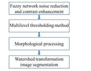
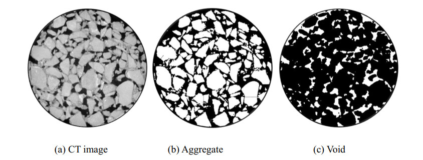
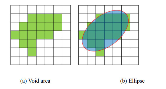
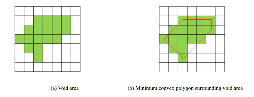
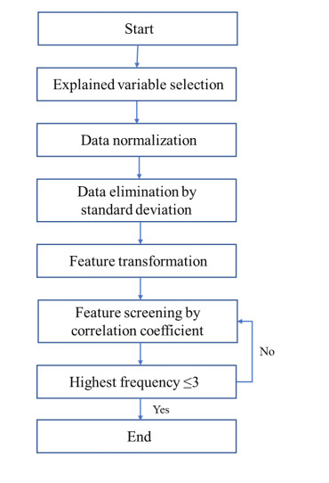
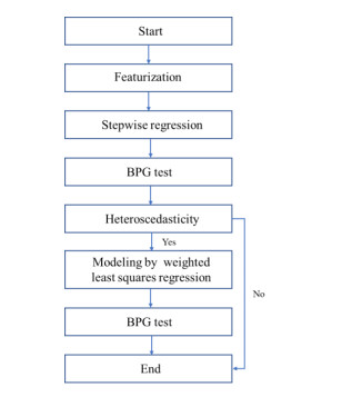
1.   Introduction

Asphalt mixture is a multiphase composite material composed of aggregate, asphalt and mineral powder. There are wide variations for the physical and mechanical properties in different kinds of asphalt mixtures, due to the composite gradation. The complexity and randomness of materials lead to the diversity of mesostructure and the complexity of mechanical behavior. As a bridge between gradation and macro mechanical properties, mesostructure is of great significance to reveal the influence of gradation on mechanical properties. In general, the macro performance refers to the overall performance of asphalt mixture, and the characteristics in molecular scale is defined as the micro performance. The meso scale belongs to the middle scale, and the mesostructure mainly includes aggregate, asphalt mortar and void. On the one hand, the mesostructure model of asphalt mixture used for numerical simulation needs to have a good correlation with gradation information^[1,2]; On the other hand, in pavement detection, predicting gradation information through the images of core samples can reduce the amount of test and improve the detection efficiency ^[3,4]. However, at present, the correlation model between mesostructure and gradation is relatively simple, less influencing factors are considered, and there is a lack of statistical model, which limits the application of mesostructure research results.

With the development of CT technology, it provides an important approach to study the mesostructure of asphalt mixture. The mesostructure CT images can be accurately identified and segmented to obtain the aggregate, asphalt mortar and void by digital image processing technology ^[5,6,7,8]. For the study of void characteristics, the plane and spatial distribution of voids are mainly studied. Wang Linbing ^[9] obtained the internal images of asphalt mixture from the Westrack test road by the industrial CT, and extracted the void spatial distribution and size information to evaluate the mesostructure property of asphalt mixture. Masad ^[10] concluded that the spatial distribution of void size in asphalt mixture showed a trend of larger at both ends and smaller in the middle. Compaction mode and aggregate size had a great impact on void size distribution. Xu Huining ^[11] put forward the parameters such as void fraction, tortuosity and average void diameter, and revealed the change of void distribution characteristics during freeze-thaw cycles. Further study ^[12] obtained the influence of void structure on water seepage in asphalt mixture. Arambula ^[13] obtained the void distribution in the depth direction of asphalt mixture with different gradation and compaction method and established the relationship between void and water stability. Jiang Wei ^[14] put forward the evaluation indexes of void quantity and area. The research showed that the meso void distribution characteristics were greatly affected by gradation and maximum nominal particle size, and the equivalent void diameter had a good correlation with the permeability, sound absorption and shear strength of asphalt mixture.

As the main load bearing structure of asphalt mixture, the spatial distribution of aggregate directly affects the service performance ^[15,16,17]. Industrial CT can extract the information of aggregates in asphalt mixture, and then obtain its position and volume. Yue ^[18] analyzed the quantitative measurement results of coarse aggregate distribution and shape in dense asphalt mixture, and found that the main axis direction has a trend of horizontal distribution. Gopalakrishnan ^[19] extracted the nearest distance between aggregates and measured the change of distance during compaction. Coenen ^[20] defined the contact distance threshold through the relationship between the contact distance and the number of contact points, and then determined the number of contact points as the evaluation index of the skeleton structure. Sefidmazgi ^[21] proposed aggregate contact evaluation indexes such as the number of contact points, contact line length and contact plane direction, and proved that aggregate contact have a good correlation with the rutting resistance.

It can be seen from the above that at present, the research on the mesostructure of asphalt mixture is carried out from the aspects of morphology and distribution of void and aggregate. However, each study only focuses on a small number of gradation, and there is a lack of statistical relationship model between mesostructure and gradation. Therefore, this study obtains a large number of mesostructure images of asphalt mixture with different gradation through industrial CT, extracts mesostructure parameters, and then establishes the relationship between gradation and mesostructure through the statistical methods. The research objective of this paper is to accurately predict the meso structure and gradation, mainly including two aspects:

1) In the road detection process, it is necessary to obtain the gradation information of a section of the road. The gradation can be predicted by the images of the core sample of the road.

2) In order to accurately establish the mesostructure discrete element model of asphalt mixture ^[22,23,24], the mesostructure parameters should be accurately predicted by gradation.

2.   Materials and test method

2.1.   Properties of materials

In this study, andesite from Heilongjiang province, limestone powder from Jilin Province and 90# neat asphalt are used. Materials tests are carried out according to JTG E42-2005 Test Methods of Aggregate for Highway Engineering and JTGF40-2004 Technical Specification for Construction of Highway Asphalt Pavements. The properties of materials are shown in Tables 1-3.

2.2.   Gradation of asphalt mixture

In order to improve the accuracy of prediction results, a large number of CT scanning specimens are needed. By adjusting the proportion of coarse and fine aggregate, 66 gradations are selected in this research. Two repetitions are manufactured for each gradation, and a total of 132 specimens are scanned by CT. The 66 gradations are shown in Table 4.

It can be seen from Table 4 that the gradations cover different types of asphalt mixture and maximum nominal aggregate size, and there are big differences between gradations. By Marshall design method, the optimal asphalt contents are obtained according to JTGF40-2004 Technical Specification for Construction of Highway Asphalt Pavements. The gradation coverage is relatively wide, which can also ensure the accuracy of mesostructure parameters prediction.

2.3.   Computed tomography scan and digital image processing method

The CT scanning equipment used for asphalt mixture samples is the micro focus industrial CT owned by Harbin Institute of Technology. Both cone beam scanning system and cone beam filter back projection reconstruction algorithm are applied to reconstruct the images. The scanning voltage/current is 195 kv/95μA.

Through CT scanning, the cross section images of asphalt mixture specimens can be obtained, and 400 images are extracted from each specimen. These images are the basis for extracting the mesostructure parameters of asphalt mixture. At present, the most used method to extract the mesostructure of asphalt mixture is digital image processing technology. The research team also proposed an image processing method ^[4] used in this research, as shown in the Figure 1.

3.   Methodology of mesostructure parameters extraction and modelling

Typical asphalt mixture images are shown in the Figure 2(a). The size of the image is 1000 pixels × 1000 pixels. It can be seen that asphalt mixture mainly includes aggregates and voids on the meso scale as shown in Figure 2(b), (c). The simple mesostructure parameters include the area of voids and aggregates, and the complex parameters include the shape of voids and aggregate contact. Based on the summary of existing literature and previous research results of our research group, 14 void parameters and 12 aggregate parameters in meso scale are list in this paper. These mesostructure parameters are directly related to the gradation of asphalt mixture, and the void and aggregate parameters will be introduced in detail below.

3.1.   Mesostructure parameters of void

1) Number of voids

Void area

The number of all pixels in the void position in the image, and the unit need to be converted to metric system as mm².

2) Ratio of void area to cross-sectional area of specimen

The sum of the areas of all voids in the image can be divided by the cross-sectional area of the specimen to obtain the parameter.

where Area_i is area of the i^th void area, p is the number of voids, S is the cross-sectional area of the specimen.

3) Centroid coordinates of void

The abscissa of the centroid coordinate of the void is the average value of the abscissas of all pixels constituting the void area, and the ordinate calculation method is the same as above. The calculation methods are shown as Eqs (2) and (3).

where X_i and Y_i are the centroid coordinates of the NO.i void area, n_i is the number of pixels in the i^th void area, x_{i, j} and y_{i, j} are the abscissa and ordinate of the j^th pixel in the i^th void area.

4) Equivalent circle radius of void

First, the area of the void should be determined, and then the area is used to deduce the radius of the circle with the same area as the void, as shown in Eq (4).

where Ri is the equivalent circle radius of the i^th void area, Area_i is the area of the i^th void.

5) Circumscribed rectangular area and ratio of the rectangular area to void area

For getting the circumscribed rectangle of the closed area, the abscissa and ordinate values of all pixels in the void area should be extracted, and then the circumscribed rectangle can be determined by the maximum and minimum values of abscissa and ordinate, as shown in Figure 3.

After the circumscribed rectangular is determined, the calculation formulas of circumscribed rectangular area and ratio of the rectangular area to void area are shown in Eq (5) and (6).

where Area_{i, rectangle} is the circumscribed rectangular area of the i^th void area, x_{i, max}, x_{i, min} are the maximum and minimum abscissa values of pixels in the i^th void area, y_{i, max}, y_{i, min} are the maximum and minimum ordinate values of pixels in the i^th void area, Ratio_{i, rectangle} is the ratio of the circumscribed rectangular area to the i^th void area.

6) Perimeter of void

The calculation of void perimeter is based on the identification of the edge of the closed area. After identifying the edge of the closed area, the connecting line length of the pixel center of the edge pixel is the perimeter of the void, as shown in Figure 4. The calculation method is shown as Eq (7).

where Ci is the perimeter of the i^th void area, mi is the number of edge pixels of the i^th void area, x_{i, k}, y_{i, k}, x_{i, k+1}, y_{i, k+1} are the abscissa and ordinate values of kth and k+1 th pixels on the edge of the i^th void area.

7) Center of void edge

The edge is divided into mi segments. The abscissa and ordinate of the starting point of each segment are weighted by its segment length. Finally, and then it is divided by the edge perimeter to calculate the center of void edge. The calculation formula is shown in Eqs (8) and (9).

where X_{i, edge} and Y_{i, edge} are the abscissa and ordinate of the edge center of the i^th void area, mi is the number of edge pixels of the i^th void area, x_{i, k} and y_{i, k} are the abscissa and ordinate of the kth pixel on the edge of the i^th void area, x_{i, k+1} and y_{i, k+1} are the abscissa and ordinate of the k+1^th pixel on the edge of the i^th void area.

8) Average distance from void edge to center of void edge

Based on the center information of void edge, the average distance from the void edge to the center can be further calculated, as shown in Eq (10).

where D_{i, edge} is average distance from void edge to center, Δ_{si, k} is the distance between the kth edge point and the k+1st edge point of the i^th void area.

9) The variance of distance between void edge to center of void edge

The parameter can be calculated by Eq (11), and it can be used to characterize the dispersion of edge pixels.

10) Gaussian descriptors of voids

Gaussian descriptors are invariant to translation, transformation and scaling. The calculation formulas of Gaussian descriptors are shown as Eqs (12) and (13).

where $I(\lambda)$ is Gaussian descriptors, $f(\theta, \lambda)$ is Gaussian potential function. K is the number of copies divided equally at 360 degrees, and K is generally taken as 3-8. In order to extract the difference of details as much as possible, K = 8 is taken in this study. In order to extract enough information to characterize shape features, $\lambda$ takes 8 different values, namely: 0.25D_{i, edge}, 0.5 D_{i, edge}, 0.75 D_{i, edge}, D_{i, edge}, 1.25 D_{i, edge}, 1.5 D_{i, edge}, 1.75D_{i, edge}, 2 D_{i, edge}.

11) Length of major and minor axes of ellipse with the same standard second-order central moment as the void

The relation between void area and ellipse is shown in Figure 5. The calculation formula for the parameter is shown in Eqs (14)-(17).

where u_xx, u_yy are the variances of abscissa and ordinate of void area, u_xy is the covariance of abscissa and ordinate of void area. λ₁ and λ₂ are eigenvalues. a and b are the lengths of major and minor axes of ellipse.

12) Eccentricity of ellipse with the same standard second-order central moment as the void

To calculate the eccentricity of the ellipse, the half focal length of the ellipse should be calculated firstly. The calculation method is shown as Eq (18) and (19).

where c is the half focal length of ellipse, e is the eccentricity of ellipse.

13) Area of convex polygon surrounding void

Firstly, the minimum convex polygon surrounding the void area should be determined, and then the number of pixels in the convex polygon can be obtained. The calculation method is shown in Figure 6.

14) The ratio of void area to the number of pixels at the edge of the void

where Ratio_{i, edge} is the ratio of the i^th void area to the number of pixels at the edge of the i^th void.

3.2.   Mesostructure parameters of aggregate

Before calculating the aggregate parameters, it is necessary to classify the aggregate size. The width of the smallest circumscribed rectangle of the aggregate is taken as the size of the aggregate. In the CT image of asphalt mixture, it is obvious that the voids are black, and the aggregate and asphalt are gray. Therefore, it is easy to extract voids by digital image processing method. However, for the separation of aggregate and asphalt, it is difficult to distinguish the aggregates smaller than 0.6 mm from asphalt. For the current CT scanning accuracy and digital image processing algorithm, only the aggregate larger than 0.6 mm can be accurately extracted. Since it is difficult to identify aggregates smaller than 0.6 mm by image processing, the aggregates sizes are classified as: greater than 19 mm, 19-16 mm, 16-13.2 mm, 13.2-9.5 mm, 9.5-4.75 mm, 4.75-2.36 mm, 2.36-1.18 mm and 1.18-0.6 mm.

Based on the aggregate classification above, the following aggregate parameters are calculated for each grade of aggregate.

1) Number of each grade aggregate

2) Proportion of quantity of each grade aggregate in the total

3) Total area of aggregate

4) Area of each grade aggregate

5) Proportion of area of each grade aggregate in the total

6) Mean value of average distance between aggregate centroids for each grade aggregates

The parameters can be calculated by Eq (21).

where D_{mean, i} is the average value of the distance between the centroid of i^th aggregate and the other aggregates for the same grade. D_mean is mean value of average distance between aggregate centroids for each grade aggregates. n is the number of aggregates for a certain grade.

7) Mean value of minimum distance between aggregate centroids for each grade

This parameter can evaluate the local distribution of aggregates in the mixture, and the parameters can be calculated by Eq (22).

where D_{min, i} is the minimum distance between the centroid of i^th aggregate and the other aggregates for the same grade. D_mean is mean value of minimum distance between aggregate centroids for each grade aggregates. n is the number of aggregates for a certain grade.

8) Mean value of the minimum distance between the edges of aggregates for the same grade

The parameter is calculated by subtract the sum of the equivalent circle radius of the two aggregates from the distance between the two aggregate centroids.

where D_{edge, i} is the minimum distance between the edge of i^th aggregate and that of the other aggregate for the same grade. D_edge is the average of Dedge, i of all the aggregate. r_i is the equivalent circle radius of the i^th aggregate. r_j is the equivalent circle radius of the j^th aggregate. n is the number of aggregates for a certain grade.

9) Area ratio of different grade aggregates

This parameter is mainly used to characterize the distribution state of small aggregates around a large aggregate. A circle is draw with the centroid of aggregate i and radius Dmin. m aggregates smaller than the grade which aggregate i belongs to is counted. The calculation method is shown in Eq (24).

where S_j is the area of the j^th small aggregate within D_min around aggregate i, S_small is the total area of the small aggregates, Area_i is the area of aggregate i, Si is the area ratio of aggregate i, S_ratio is the average of Si of all the n aggregate in a certain grade. n is the number of aggregates for a certain grade.

10) Number of small aggregate in the range of minimum distance between centroids

The parameter is the number of aggregates in the circle drawn in the previous step, and it can characterize the distribution of small aggregates around a large aggregate.

11) Ratio of aggregate area to cross-sectional area of specimen

The sum of the areas of all aggregates in the image can be divided by the cross-sectional area of the specimen to obtain the ratio.

where Ratio_aggregate is the ratio of aggregate area to cross-sectional area of specimen. n is the number of aggregates in the image. S is the cross-sectional area of specimen.

12) Ratio of asphalt mortar area to cross-sectional area of specimen

The mortar area is equal to the cross section area minus the void area and aggregate area, and then the parameter can be calculated.

3.3.   Sampling and featurization

For each gradation, 800 images can be obtained from the two specimens, and the average value and standard deviation of the meso structure parameters of 800 image samples can be calculated. Before modeling, featurization needs to be carried out. The featurization is to find and screen better features to join the model to improve the performance of the model. The process is shown as follow:

1) Explained variable selection

2) Feature filtering based on standard deviation

The data of the feature pool is transformed to [-1, 1], and the standard deviation of each feature in all samples is calculated. After repeated trials, it is found that when the standard deviation threshold is 0.4, the remaining features in the final screening can be roughly about 20. In order to simplify the calculation, the threshold is set to 0.4, and the features with standard deviation less than 0.4 are removed.

3) Feature transformation

Data transformation is carried out for the remaining features, that is, x is transformed into five forms: x, x², ln (x + 1), x^0.5 and 1/(x + 1). Because the relationship between features and explained variables is not necessarily linear, for establishing a linear model, the relationship between features and explained variables needs to be modified into a linear relationship. The absolute value of the correlation coefficient between the transformed data and the explained variable is used to judge the data transformation of the feature finally. The transformation form with the highest correlation coefficient will be retained. This step does not increase or reduce the features, but only changes the data form of the feature.

4) Screening based on correlation coefficient between features

To ensure the independence between features, the correlation coefficient matrix between features is calculated, and the absolute value of the matrix is obtained. The frequency of the absolute value of correlation coefficient between each feature and other features is greater than 0.6 is counted. The features with the highest frequency are removed and iterated successively until the highest frequency is less than or equal to 3.

Through the above featurization method, on the one hand, it can greatly reduce the interference of features with low correlation, on the other hand, it can improve the quality of features and lay a good foundation for the correlation models.

3.4.   Gradation prediction model by mesostructure parameters

Forward stepwise regression method are utilized for predicting gradation through mesostructure with the P-value of 0.05. The reason why stepwise regression rather than machine learning method is adopted here is that if the neural network model is constructed, its input and output scale is in double digits, and the constructed network scale is too large compared with 64 groups of samples. It is not suitable to use machine learning method for modeling.

The essence of forward stepwise regression is OLS (Ordinary Least Square Method), but stepwise regression is a method combining multiple OLS. Its purpose is to find the most appropriate explanatory variable and add it to the equation. The specific steps are as follows:

1) Unary linear regression is performed between explanatory variable (X₁, X₂...) and explained variable (Y), and the F-statistics of each regression equation are calculated as (F₁¹, F₂¹...). For the maximum value F_i¹, the critical value is F¹ at the significance level α. If F_i¹ ≥ F¹, Xi is introduced into the equation.

2) Binary linear regression is performed between explanatory variable ((X₁, X_i), (X₂, X_i)...) and explained variable (Y), and the F-statistics of each regression equation are calculated as (F₁², F₂²...). For the maximum value F_j², the critical value is F² at the significance level α. If F_j² ≥ F², X_j is introduced into the equation.

3) More explanatory variables are introduced until the maximum F-statistic is less than the critical value, that is, the end of stepwise regression.

The explained and explanatory variables are shown in Tables 5 and 6.

In the modeling process, 8 grades of aggregates, 102 mesostructure parameters, 64 gradation (128 specimens) are utilized. The modeling process is as follows:

1) Firstly, based on the explained variables, the featurization is performed to screen the explanatory variables.

2) The filtered explanatory variables are imported into the stepwise regression model for modeling.

3) Breusch-Pagan-Godfrey (BPG) test is carried out on the established model to test whether there is heteroscedasticity problem.

4) If there is heteroscedasticity problem, weight should be calculated to modeling by the weighted least squares regression. Otherwise, the modeling is completed.

The modeling process are shown in Figure 8.

Since the process of modeling the passing percentage of each sieve are similar, the modeling of the passing percentage on the 1.18 mm sieve is selected for detailed introduction, and the rest are briefly displayed.

4.   Results and discussion

4.1.   Gradation prediction model by mesostructure parameters

4.1.1.   Modeling of Passing percentage on 1.18 mm sieve

The explained variable is selected as the passing percentage on 1.18 mm sieve (P_1.18), and the featurization is carried out on the feature pool. Finally, there are 20 remaining features. All features are normalized, and stepwise regression is carried out to obtain the model:

When the significance level is 0.05, the adjoint probability of F-statistic is less than 0.05, that is, the equation is significant.

For the BPG test, the OLS regression is performed on the logarithm of the square term of the residual and the independent variable, and the pro (F-statistic) is 0.023. Under the significance level of 0.05, the original assumption that the equation is not significant is rejected, that is, there is a heteroscedasticity.

In order to solve the heteroscedasticity problem, the original independent variables are retained, and the weighted least square method is used for regression. Firstly, the weight of each independent variable is calculated. After trial calculation, it is found that the following formula has high goodness of fit, R² = 0.335.

The weight is calculated by above formula, and the weighted least square method is used for regression. The new model is shown as Eq (28).

The BPG test is performed again, and it is found that the adjoint probability of F-statistic is 0.635. Under the significance level of 0.05, the original hypothesis is accepted, that is, there is no heteroscedasticity.

4.1.2.   Modeling of Passing percentage for other sieves

1) Modeling of Passing percentage on 19 mm sieve

2) Modeling of Passing percentage on 16 mm sieve

3) Modeling of Passing percentage on 13.2 mm sieve

4) Modeling of Passing percentage on 9.5 mm sieve

5) Modeling of Passing percentage on 4.75 mm sieve

6) Modeling of Passing percentage on 2.36 mm sieve

7) Modeling of Passing percentage on 0.6 mm sieve

8) Modeling of CA ratio

9) Modeling of FA ratio

4.2.   Mesostructure parameter prediction model by gradation

Because there are too many mesostructure parameters, modeling all the parameters will make the article lengthy. Therefore, the average distance between aggregates of 9.5-4.75 mm is selected for modeling in this study.

There are 800 mesostructure images for each gradation, therefore the mesostructure indexes predicted by gradation are a range instead of a fixed value. The difference is characterized by mean and standard deviation. The explained variables and explanatory variables are shown in Tables 7 and 8.

(i) Modeling of AD_mean(9.5-4.75 mm)

Feature engineering is carried out on the feature pool, and 10 features are finally left. Normalization and stepwise regression are carried out for all features, and the following model is obtained:

At the significance level of 0.05, the concomitant probability of F-statistic is less than 0.05, that is, the null hypothesis that all structural parameters are significantly 0 is rejected, and the equation is significant.

For the BPG test, OLS regression is performed on the square term of residuals and independent variables. Significance test is performed on the equation to check whether heteroscedasticity existed. The test Pro(F-statistic) was 0.278. At the significance level of 0.05, the null hypothesis that the equation is not significant is accepted, that is, there is no heteroscedasticity.

(ii) Modeling of SD_AD

Feature engineering is carried out on the feature pool, and 10 features are finally left. Normalization and stepwise regression are carried out for all features, and the following result is obtained:

When the significance level is 0.05, the adjoint probability of F statistic is less than 0.05. The original assumption that all structural parameters are significant is 0 is rejected, that is, the equation is significant.

For the BPG test, OLS regression is performed on the square term of residual and independent variables. The equation significance test is performed on the equation to check whether there is heteroscedasticity problem. The F-statistic is 0.013. Under the significance level of 0.05, the original hypothesis that the equation is not significant is rejected, that is, there is heteroscedasticity.

In order to solve the heteroscedasticity problem, the original independent variables are retained, and the weighted least square method is used for regression. Firstly, the weight of each independent variable is calculated. After trial calculation, it is found that the following formula has high goodness of fit, R² = 0.683.

The weight is calculated by the above formula, and the weighted least square method is used for regression to obtain:

The BPG test is performed again. It is found that the adjoint probability of F statistic is 0.415. Under the significance level of 0.05, the original hypothesis is accepted, that is, there is no heteroscedasticity.

4.3.   Model verification

An example is added to demonstrate the use scenario of the above model. The model examples established in Sections 4.2 and 4.3 are demonstrated respectively. The calculation example of the mesostructure parameters prediction based on gradation adopts the model of predicting the passing percentage of the 4.75 mm sieve. For the gradation prediction, the mean value of average distance between aggregate centroids for 9.5-4.75 mm aggregates is used as an example.

4.3.1.   Prediction of the passing percentage of the 4.75 mm sieve

Background: in the road detection process, it is necessary to obtain the gradation information of a section of the road.

1) Obtaining sectional image

The core sample of the pavement is cut to obtain 10 section images at different positions. The purpose is to make the average value of the calculated mesostructure parameters more stable, that is, the average value can better represent the state of the core sample.

2) Image processing and calculation of mesostructure parameters

The image processing method developed in this research is used to process 10 cross section images, and 10 void images and aggregate images are obtained respectively. These images are imported to the calculation program the obtain the mesostructure parameters, and 7 parameters are extracted from the mesostructure parameters system as Eq (33). The parameters are shown in Table 9.

3) Data preprocessing

Based on the prediction model, the data transformation is performed. According to the maximum and minimum value of the mesostructure parameter database, the data is normalized. The preprocessed date is shown in Table 10.

4) Calculation of prediction results

The above values are substituted into Eq (33) to calculate the passing percentage of the 4.75 mm sieve as shown in Eq (42).

Finally, the prediction passing percentage of 4.75 mm sieve is 33.8841%, while the actual value used in this example is 30%. The prediction error is acceptable.

4.3.2.   Predicted average distance between 9.5-4.75 mm aggregate

Background: the gradation of asphalt mixture is known, and the corresponding mesostructure parameters should be analyzed.

1) Gradation data processing

Firstly, gradation is converted into the mass percentage on the sieve, and then the aggregate smaller than 0.6 mm is removed to calculate the mass percentage on the other sieves.

As in the previous example, the data transformation and normalization are performed. The data for mean value and standard deviation are shown in Tables 12 and 13.

2) Calculate the mean and standard deviation

The data in Table 12 is substituted into Eq (38) to calculate the mean value.

The data in Table 13 is substituted into Eq (39) to calculate the standard deviation:

The mean value is 46.8507 and the standard deviation is 2.1194.

3) Calculate the confidence interval of mesostructure parameters

Based on the t-distribution table, when the significance level is 0.1 and 800 samples, the value of t-statistic is 1.645. It is substituted into the following formula to calculate the confidence interval:

The confidence interval for predicting the average distance between 9.5-4.75 mm aggregates is [46.7274, 46.9739].

In this paper, the prediction of mesostructure parameter and gradation are of great significance for future construction gradation identification and digital modeling. However, this paper also has some limitations, which are mainly reflected in the following two aspects:

1) At present, the gradation identification ability of asphalt mixture is limited, which makes it difficult to accurately identify aggregates with the diameter smaller than 1.18 mm;

2) Although we have 132 specimens by CT scan at present, it is still difficult to meet the requirements of accurate prediction. In the future, we will continue to expand the amount of data and improve the prediction accuracy of the model.

5.   Conclusions

In this paper, the mesostructure images of asphalt mixtures with 64 gradations are obtained by industrial CT, and the meso structure parameters are extracted. The correlation models between gradation and mesostructure parameters are established and verified based on econometric method. The conclusions can be drawn as follows:

1) Based on digital image processing method, void and aggregate parameters are extracted from 64 types of asphalt mixtures. At the same time, gradation parameters are proposed, including percentages retaining on sieve, CA ratio and FA ratio. 102 mesostructure parameters and 10 gradation parameters are selected for modeling.

2) Featurization used in this paper including data augmentation, standard deviation screening and correlation coefficient screening. The feature quality after featurization is greatly improved and the number of explanatory variables of the model can be reduced.

3) According to featurization and stepwise regression, the gradation prediction models based on mesostructure parameters are established. The econometric hypothesis test is carried out on the models. For the models with heteroscedasticity, the weighted least square regression is used to solve the heteroscedasticity problem.

4) The passing percentage of the 4.75 mm sieve and the mean value of average distance between aggregate centroids for 9.5-4.75 mm aggregates are used as examples. The prediction error of passing percentage is acceptable, and the confidence interval of mesostructure parameters are also given.

Acknowledgments

This paper was supported by National Key Research and Development Program of China (No. 2022YFB2602600), National Natural Science Foundation of China (No. 51908168), Postdoctoral Science Foundation of China (No. 2019M651192 and No. 2020T130150), Heilongjiang Postdoctoral Fund (No. LBH-Z19163). All data, models, and code generated or used during the study appear in the published article.

Conflicts of interest

The authors declare no conflicts of interest.