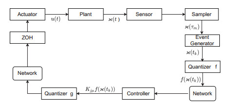
This paper investigates the issue of asynchronous $ H_{\infty} $ tracking control for nonlinear semi-Markovian jump systems (SMJSs) based on the T-S fuzzy model. Firstly, in order to improve the performance of network control systems (NCSs) and the efficiency of data transmission, this paper adopts a double quantization strategy which quantifies the input and output of the controllers. Secondly, for the purpose of reducing the burden of network communication, an adaptive event-triggered mechanism (AETM) is adopted. Thirdly, due to the influence of network-induce delay, the system mode information can not be transmitted to the controller synchronously, thus, a continuous-time hidden Markov model (HMM) is established to describe the asynchronous phenomenon between the system and the controller. Additionally, with the help of some improved Lyapunov-Krasovski (L-K) functions with fuzzy basis, some sufficient criteria are derived to co-guarantee the state stability and the $ H_{\infty} $ performance for the closed-loop tracking control system. Finally, a numerical example and a practical example are given to verify the effectiveness of designed mentality.
Citation: Yuxin Lou, Mengzhuo Luo, Jun Cheng, Xin Wang, Kaibo Shi. Double-quantized-based $ H_{\infty} $ tracking control of T-S fuzzy semi-Markovian jump systems with adaptive event-triggered[J]. AIMS Mathematics, 2023, 8(3): 6942-6969. doi: 10.3934/math.2023351
This paper investigates the issue of asynchronous $ H_{\infty} $ tracking control for nonlinear semi-Markovian jump systems (SMJSs) based on the T-S fuzzy model. Firstly, in order to improve the performance of network control systems (NCSs) and the efficiency of data transmission, this paper adopts a double quantization strategy which quantifies the input and output of the controllers. Secondly, for the purpose of reducing the burden of network communication, an adaptive event-triggered mechanism (AETM) is adopted. Thirdly, due to the influence of network-induce delay, the system mode information can not be transmitted to the controller synchronously, thus, a continuous-time hidden Markov model (HMM) is established to describe the asynchronous phenomenon between the system and the controller. Additionally, with the help of some improved Lyapunov-Krasovski (L-K) functions with fuzzy basis, some sufficient criteria are derived to co-guarantee the state stability and the $ H_{\infty} $ performance for the closed-loop tracking control system. Finally, a numerical example and a practical example are given to verify the effectiveness of designed mentality.

| [1] |
Q. T. Jiang, X. H. Zhou, R. L. Wang, W. P. Ding, Y. Chu, S. Z. Tang, et al., Intelligent monitoring for infectious diseases with fuzzy systems and edge computing: a survey, Appl. Soft Comput., 123 (2022), 108835. https://doi.org/10.1016/j.asoc.2022.108835 doi: 10.1016/j.asoc.2022.108835

|
| [2] |
D. Dell'Anna, A. Jamshidnejad, Evolving fuzzy logic systems for creative personalized socially assistive robots, Eng. Appl. Artif. Intel., 114 (2022), 105064. https://doi.org/10.1016/j.engappai.2022.105064 doi: 10.1016/j.engappai.2022.105064
|
| [3] |
Y. J. Liu, X. Y. Zhao, J. H Park, F. Fang, Fault-tolerant control for T-S fuzzy systems with an aperiodic adaptive event-triggered sampling, Fuzzy Sets Syst., 452 (2022), 23–41. https://doi.org/10.1016/j.fss.2022.04.019 doi: 10.1016/j.fss.2022.04.019
|
| [4] |
P. Shi, F. B. Li, L. G. Wu, C. Lim, Neural network-based passive filtering for delayed neutral-type semi-Markovian jump systems, IEEE Trans. Neural Networks Learn. Syst., 28 (2017), 2101–2114. https://doi.org/10.1109/TNNLS.2016.2573853 doi: 10.1109/TNNLS.2016.2573853
|
| [5] |
Y. L. Wei, J. H. Park, J. B. Qiu, L. G. Wu, H. Y. Jung, Sliding mode control for semi-Markovian jump systems via output feedback, Automatica, 81 (2017), 133–141. https://doi.org/10.1016/j.automatica.2017.03.032 doi: 10.1016/j.automatica.2017.03.032
|
| [6] |
H. Shen, F. Li, S. Y. Xu, V. Sreeram, Slow state variables feedback stabilization for semi-Markov jump systems with singular perturbations, IEEE Trans. Automat. Control, 63 (2018), 2709–2714. https://doi.org/10.1109/TAC.2017.2774006 doi: 10.1109/TAC.2017.2774006
|
| [7] |
X. Xing, D. Y. Yao, Q. Lu, X. C. Li, Finite-time stability of Markovian jump neural networks with partly unknown transition probabilities, Neurocomputing, 159 (2015), 282–287. https://doi.org/10.1016/j.neucom.2015.01.033 doi: 10.1016/j.neucom.2015.01.033
|
| [8] |
Z. L. Xia, S. P. He, Finite-time asynchronous $H_{\infty}$ fault-tolerant control for nonlinear hidden Markov jump systems with actuator and sensor faults, Appl. Math. Comput., 428 (2022), 127212. https://doi.org/10.1016/j.amc.2022.127212 doi: 10.1016/j.amc.2022.127212
|
| [9] |
T. Wu, L. L. Xiong, J. D. Cao, J. H. Park, Hidden Markov model-based asynchronous quantized sampled-data control for fuzzy nonlinear Markov jump systems, Fuzzy Sets Syst., 432 (2022), 89–110. https://doi.org/10.1016/j.fss.2021.08.016 doi: 10.1016/j.fss.2021.08.016
|
| [10] |
F. Li, S. Y. Xu, B. Y. Zhang, Resilient asynchronous $H_{\infty}$ control for discrete-time Markov jump singularly perturbed systems based on hidden Markov model, IEEE Trans. Syst. Man Cybern. Syst., 50 (2020), 2860–2869. https://doi.org/10.1109/TSMC.2018.2837888 doi: 10.1109/TSMC.2018.2837888
|
| [11] |
Z. H. Xiao, Z. Y. Wu, J. Tao, Asynchronous filtering for Markov jump systems within finite time: a general event-triggered communication, Commun. Nonlinear Sci. Numer. Simul., 114 (2022), 106634. https://doi.org/10.1016/j.cnsns.2022.106634 doi: 10.1016/j.cnsns.2022.106634
|
| [12] |
D. Zhang, C. Deng, G. Feng, Resilient cooperative output regulation for nonlinear multi-agent systems under DoS attacks, IEEE Trans. Automat. Control, 2022, 1–8. https://doi.org/10.1109/TAC.2022.3184388 doi: 10.1109/TAC.2022.3184388
|
| [13] |
L. G. Wu, Y. B. Gao, J. X. Liu, H. Y. Li, Event-triggered sliding mode control of stochastic systems via output feedback, Automatica, 82 (2017), 79–92. https://doi.org/10.1016/j.automatica.2017.04.032 doi: 10.1016/j.automatica.2017.04.032
|
| [14] |
Z. D. Lu, G. T. Ran, F. X. Xu, J. X. Lu, Novel mixed-triggered filter design for interval type-2 fuzzy nonlinear Markovian jump systems with randomly occurring packet dropouts, Nonlinear Dyn., 97 (2019), 1525–1540. https://doi.org/10.1007/s11071-019-05070-x doi: 10.1007/s11071-019-05070-x
|
| [15] |
H. Shen, M. S. Chen, Z. G. Wu, J. D. Cao, J. H. Park, Reliable event-triggered asynchronous extended passive control for semi-Markov jump fuzzy systems and its application, IEEE Trans. Fuzzy Syst., 28 (2020), 1708–1722. https://doi.org/10.1109/TFUZZ.2019.2921264 doi: 10.1109/TFUZZ.2019.2921264
|
| [16] |
H. J. Wang, A. K. Xue, J. H. Wang, R. Q. Lu, Event-based $H_{\infty}$ filtering for discrete-time Markov jump systems with network-induced delay, J. Franklin Inst., 354 (2017), 6170–6189. https://doi.org/10.1016/j.jfranklin.2017.07.017 doi: 10.1016/j.jfranklin.2017.07.017
|
| [17] |
M. Xue, H. C. Yan, H. Zhang, Z. C. Li, S. M. Chen, C. Y. Chen, Event-triggered guaranteed cost controller design for T-S fuzzy Markovian jump systems with partly unknown transition probabilities, IEEE Trans. Fuzzy Syst., 29 (2021), 1052–1064. https://doi.org/10.1109/TFUZZ.2020.2968866 doi: 10.1109/TFUZZ.2020.2968866
|
| [18] |
Z. H. Ye, D. Zhang, J. Cheng, Z. G. Wu, Event-triggering and quantized sliding mode control of UMV systems under DoS attacks, IEEE Trans. Veh. Tech., 71 (2022), 8199–8211. https://doi.org/10.1109/TVT.2022.3175726 doi: 10.1109/TVT.2022.3175726
|
| [19] |
L. Su, G. Chesi, Robust stability of uncertain discrete-time linear systems with input and output quantization, IFAC-PapersOnLine, 50 (2017), 375–380. https://doi.org/10.1016/j.ifacol.2017.08.161 doi: 10.1016/j.ifacol.2017.08.161
|
| [20] |
L. L. Su, G. Chesi, Robust stability of uncertain linear systems with input and output quantization and packet loss, Automatica, 87 (2018), 267–273. https://doi.org/10.1016/j.automatica.2017.10.014 doi: 10.1016/j.automatica.2017.10.014
|
| [21] |
H. J. Tang, X. M. Zhang, H. Zhu, J. Lv, Quantized feedback control for time-delay systems via sliding mode observers, IMA J. Math. Control Inform., 35 (2018), 1–23. https://doi.org/10.1093/imamci/dnw014 doi: 10.1093/imamci/dnw014
|
| [22] |
J. H. Wang, Q. L. Zhang, F. Bai, Robust control of discrete-time singular Markovian jump systems with partly unknown transition probabilities by static output feedback, Int. J. Control Automat. Syst., 13 (2015), 1313–1325. https://doi.org/10.1007/s12555-014-0290-2 doi: 10.1007/s12555-014-0290-2
|
| [23] |
S. C. Zhang, B. Zhao, D. R. Liu, Y. W. Zhang, Observer-based $H_{\infty}$ tracking control scheme and its application to robot arms, IFAC-PapersOnLine, 53 (2020), 536–541. https://doi.org/10.1016/j.ifacol.2021.04.199 doi: 10.1016/j.ifacol.2021.04.199
|
| [24] |
D. Cui, Y. Wang, H. Y. Su, Z. W. Xu, H. Y. Que, Fuzzy-model-based tracking control of Markov jump nonlinear systems with incomplete mode information, J. Franklin Inst., 358 (2021), 3633–3650. https://doi.org/10.1016/j.jfranklin.2021.02.039 doi: 10.1016/j.jfranklin.2021.02.039
|
| [25] |
S. Harshavarthini, O. M. Kwon, S. M. Lee, Uncertainty and disturbance estimator-based resilient tracking control design for fuzzy semi-Markovian jump systems, Appl. Math. Comput., 426 (2022), 127123. https://doi.org/10.1016/j.amc.2022.127123 doi: 10.1016/j.amc.2022.127123
|
| [26] |
Z. H. Ye, D. Zhang, Z. G. Wu, H. C. Yan, A3C-based intelligent event-triggering control of networked nonlinear unmanned marine vehicles subject to hybrid attacks, IEEE Trans. Intell. Transp. Syst., 23 (2022), 12921–12934. https://doi.org/10.1109/TITS.2021.3118648 doi: 10.1109/TITS.2021.3118648
|
| [27] |
Z. Gu, E. G. Tian, J. L. Liu, Adaptive event-triggered control of a class of nonlinear networked systems, J. Franklin Inst., 354 (2017), 3854–3871. https://doi.org/10.1016/j.jfranklin.2017.02.026 doi: 10.1016/j.jfranklin.2017.02.026
|
| [28] |
C. Peng, T. C. Yang, Event-triggered communication and $H_{\infty}$ control co-design for networked control systems, Automatica, 49 (2013), 1326–1332. https://doi.org/10.1016/j.automatica.2013.01.038 doi: 10.1016/j.automatica.2013.01.038
|
| [29] |
A. H. Hu, J. D. Cao, M. F. Hu, L. X. Guo, Event-triggered consensus of Markovian jumping multi-agent systems via stochastic sampling, IET Control Theory Appl., 9 (2015), 1964–1972. https://doi.org/10.1049/iet-cta.2014.1164 doi: 10.1049/iet-cta.2014.1164
|
| [30] |
C. Gong, G. P. Zhu, P. Shi, Adaptive event-triggered and double-quantized consensus of leader-follower multiagent systems with semi-Markovian jump parameters, IEEE Trans. Syst. Man Cybern. Syst., 51 (2021), 5867–5879. https://doi.org/10.1109/TSMC.2019.2957530 doi: 10.1109/TSMC.2019.2957530
|
| [31] |
M. Y. Fu, L. H. Xie, The sector bound approach to quantized feedback control, IEEE Trans. Automat. Control, 50 (2005), 1698–1711. https://doi.org/10.1109/TAC.2005.858689 doi: 10.1109/TAC.2005.858689
|
| [32] |
S. Liu, T. Li, L. H. Xie, M. Y. Fu, J. F. Zhang, Continuous-time and sampled-data-based average consensus with logarithmic quantizers, Automatica, 49 (2013), 3329–3336. https://doi.org/10.1016/j.automatica.2013.07.016 doi: 10.1016/j.automatica.2013.07.016
|
| [33] |
J. S. Li, D. W. C. Ho, J. M. Li, Adaptive consensus of multi-agent systems under quantized measurements via the edge Laplacian, Automatica, 92 (2018), 217–224. https://doi.org/10.1016/j.automatica.2018.03.022 doi: 10.1016/j.automatica.2018.03.022
|
| [34] |
S. L. Hu, D. Yue, Event-triggered control design of linear networked systems with quantizations, ISA Trans., 51 (2012), 153–162. https://doi.org/10.1016/j.isatra.2011.09.002 doi: 10.1016/j.isatra.2011.09.002
|
| [35] |
M. Xue, H. C. Yan, H. Zhang, J. Sun, H. Lam, Hidden-Markov-model-based asynchronous $H_{\infty}$ tracking control of fuzzy Markov jump systems, IEEE Trans. Fuzzy Syst., 29 (2021), 1081–1092. https://doi.org/10.1109/TFUZZ.2020.2968878 doi: 10.1109/TFUZZ.2020.2968878
|
| [36] |
N. Zhao, P. Shi, W. Xing, C. P. Lim, Resilient adaptive event-triggered fuzzy tracking control and filtering for nonlinear networked systems under denial-of-service attacks, IEEE Trans. Fuzzy Syst., 30 (2022), 3191–3201. https://doi.org/10.1109/TFUZZ.2021.3106674 doi: 10.1109/TFUZZ.2021.3106674
|
| [37] | K. Gu, An integral inequality in the stability problem of time-delay systems, In: Proceedings of the 39th IEEE Conference on Decision and Control (Cat. No.00CH37187), 3 (2000), 2805–2810. https://doi.org/10.1109/CDC.2000.914233 |
| [38] |
H. K. Lam, F. H. F. Leung, Stability analysis of fuzzy control systems subject to uncertain grades of membership, IEEE Trans. Syst. Man Cybern. Part B, 35 (2005), 1322–1325. https://doi.org/10.1109/TSMCB.2005.850181 doi: 10.1109/TSMCB.2005.850181
|
| [39] |
H. K. Lam, A review on stability analysis of continuous-time fuzzy-model-based control systems: from membership-function-independent to membership-function-dependent analysis, Eng. Appl. Artif. Intell., 67 (2018), 390–408. https://doi.org/10.1016/j.engappai.2017.09.007 doi: 10.1016/j.engappai.2017.09.007
|
| [40] |
H. K. Lam, S. H. Tsai, Stability analysis of polynomial-fuzzy-model-based control systems with mismatched premise membership functions, IEEE Trans. Fuzzy Syst., 22 (2014), 223–229. https://doi.org/10.1109/TFUZZ.2013.2243735 doi: 10.1109/TFUZZ.2013.2243735
|
| [41] |
Y. N. Pan, G. H. Yang, Event-triggered fault detection filter design for nonlinear networked systems, IEEE Trans. Syst. Man Cybern. Syst., 48 (2018), 1851–1862. https://doi.org/10.1109/TSMC.2017.2719629 doi: 10.1109/TSMC.2017.2719629
|
Figures(11) / Tables(2)

Yuxin Lou, Mengzhuo Luo, Jun Cheng, Xin Wang, Kaibo Shi. Double-quantized-based $ H_{\infty} $ tracking control of T-S fuzzy semi-Markovian jump systems with adaptive event-triggered[J]. AIMS Mathematics, 2023, 8(3): 6942-6969. doi: 10.3934/math.2023351


 DownLoad: