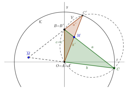
Among the triangle congruence axioms, the side-side-angle (SsA) axiom states that two triangles are congruent if and only if two pairs of corresponding sides and the angles opposite the longer sides are equal. We construct two triangle sequences in which the items satisfy a modified condition. We require that the opposite angles of the shorter sides be equal. The locus of the intersection points of other sides of triangles is derived to be a hyperbola, and in a generalized form defined by a complete quadrilateral, it is a conic section.
Citation: Peter Csiba, László Németh. Side-side-angle triangle congruence axiom and the complete quadrilaterals[J]. Electronic Research Archive, 2023, 31(3): 1271-1286. doi: 10.3934/era.2023065
Among the triangle congruence axioms, the side-side-angle (SsA) axiom states that two triangles are congruent if and only if two pairs of corresponding sides and the angles opposite the longer sides are equal. We construct two triangle sequences in which the items satisfy a modified condition. We require that the opposite angles of the shorter sides be equal. The locus of the intersection points of other sides of triangles is derived to be a hyperbola, and in a generalized form defined by a complete quadrilateral, it is a conic section.

| [1] |
J. Donnelly, The equivalence of Side–Angle–Side and Side–Angle–Angle in the absolute plane, J. Geom., 97 (2010), 69–82. https://doi.org/10.1007/s00022-010-0038-y doi: 10.1007/s00022-010-0038-y

|
| [2] |
J. Donnelly, The equivalence of Side–Angle–Side and Side–Side–Side in the absolute plane, J. Geom., 106 (2015), 541–550. https://doi.org/10.1007/s00022-015-0264-4 doi: 10.1007/s00022-015-0264-4
|
| [3] | J. F. Rigby, Congruence axioms for absolute geometry, Math Chronicle., 4 (1975), 13–44. Available from: https://www.thebookshelf.auckland.ac.nz/docs/Maths/PDF/mathschron004-003.pdf. |
| [4] |
H. Hähl, P. Peter, A variation of Hilbert's axioms for Euclidean geometry, Math. Semesterber., 69 (2022), 253–258. https://doi.org/10.1007/s00591-022-00320-3 doi: 10.1007/s00591-022-00320-3
|
| [5] | H. S. M. Coxeter, Projective Geometry, Springer, 1987. Available from: https://link.springer.com/book/9780387406237. |
| [6] | E. Fortuna, R. Frigerio, R. Pardini, Projective Geometry–-Solved Problems and Theory Review, Springer, 2016. https://doi.org/10.1007/978-3-319-42824-6 |
| [7] | Maplesoft, A division of Waterloo Maple Inc., Maple, 2022. Available from: https://www.maplesoft.com/products/. |
| [8] | P. Csiba, L. Németh, SSA Supplement Files, 2023. Available from: http://matematika.emk.uni-sopron.hu/en_GB/ssa. |


Figures(6)
Peter Csiba, László Németh. Side-side-angle triangle congruence axiom and the complete quadrilaterals[J]. Electronic Research Archive, 2023, 31(3): 1271-1286. doi: 10.3934/era.2023065


 DownLoad: