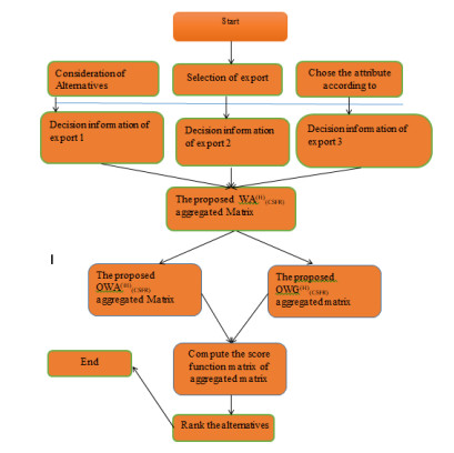
Deep learning (DL), a branch of machine learning and artificial intelligence, is nowadays considered as a core technology. Due to its ability to learn from data, DL technology originated from artificial neural networks and has become a hot topic in the context of computing, it is widely applied in various application areas. However, building an appropriate DL model is a challenging task, due to the dynamic nature and variations in real-world problems and data. The aim of this work was to develope a new method for appropriate DL model selection using complex spherical fuzzy rough sets (CSFRSs). The connectivity of two or more complex spherical fuzzy rough numbers can be defined by using the Hamacher t-norm and t-conorm. Using the Hamacher operational laws with operational parameters provides exceptional flexibility in dealing with uncertainty in data. We define a series of Hamacher averaging and geometric aggregation operators for CSFRSs, as well as their fundamental properties, based on the Hamacher t-norm and t-conorm. Further we have developed the proposed aggregation operators and provide here a group decision-making approach for solving decision making problems. Finally, a comparative analysis with existing methods is given to demonstrate the peculiarity of our proposed method.
Citation: Muhammad Ali Khan, Saleem Abdullah, Alaa O. Almagrabi. Analysis of deep learning technique using a complex spherical fuzzy rough decision support model[J]. AIMS Mathematics, 2023, 8(10): 23372-23402. doi: 10.3934/math.20231188
Deep learning (DL), a branch of machine learning and artificial intelligence, is nowadays considered as a core technology. Due to its ability to learn from data, DL technology originated from artificial neural networks and has become a hot topic in the context of computing, it is widely applied in various application areas. However, building an appropriate DL model is a challenging task, due to the dynamic nature and variations in real-world problems and data. The aim of this work was to develope a new method for appropriate DL model selection using complex spherical fuzzy rough sets (CSFRSs). The connectivity of two or more complex spherical fuzzy rough numbers can be defined by using the Hamacher t-norm and t-conorm. Using the Hamacher operational laws with operational parameters provides exceptional flexibility in dealing with uncertainty in data. We define a series of Hamacher averaging and geometric aggregation operators for CSFRSs, as well as their fundamental properties, based on the Hamacher t-norm and t-conorm. Further we have developed the proposed aggregation operators and provide here a group decision-making approach for solving decision making problems. Finally, a comparative analysis with existing methods is given to demonstrate the peculiarity of our proposed method.

| [1] | J. Karhunen, T. Raiko, K. Cho, Unsupervised deep learning: A short review, In: Advances in independent component analysis and learning machines, 2015,125–142. https://doi.org/10.1016/B978-0-12-802806-3.00007-5 |
| [2] | G. E. Hinton, S. Osindero, Y. W. Teh, A fast learning algorithm for deep belief nets, Neural Comput., 7 (2006), 1527–1554. |
| [3] |
S. A. Cohen, T. Zhuang, M. Xiao, J. B. Michaud, L. Shapiro, R. N. Kamal, Using Google Trends data to track healthcare use for hand osteoarthritis, Cureus, 13 (2021), 1–7. https://doi.org/10.7759/cureus.13786 doi: 10.7759/cureus.13786

|
| [4] | I. H. Sarker, Deep cybersecurity: A comprehensive overview from neural network and deep learning perspective, SN Comput. Sci., 3 (2021), 1–16. |
| [5] |
Y. Xin, L. Kong, Z. Liu, Y. Chen, Y. Li, H. Zhu, et al., Machine learning and deep learning methods for cybersecurity, IEEE Access, 6 (2018), 35365–35381. https://doi.org/10.1109/ACCESS.2018.2836950 doi: 10.1109/ACCESS.2018.2836950
|
| [6] |
Y. LeCun, L. Bottou, Y. Bengio, P. Haffner, Gradient-based learning applied to document recognition, P. IEEE, 86 (1998), 2278–2324. https://doi.org/10.1109/5.726791 doi: 10.1109/5.726791
|
| [7] | S. Dupond, A thorough review on the current advance of neural network structures, Ann. Rev. Control, 14 (2019). |
| [8] | D. Mandic, J. Chambers, Recurrent neural networks for prediction: Learning algorithms, architectures and stability, Wiley, 2001. |
| [9] |
P. Wei, Y. Li, Z. Zhang, T. Hu, Z. Li, D. Liu, An optimization method for intrusion detection classification model based on deep belief network, IEEE Access, 7 (2019), 87593–87605. https://doi.org/10.1109/ACCESS.2019.2925828 doi: 10.1109/ACCESS.2019.2925828
|
| [10] |
A. Aggarwal, M. Mittal, G. Battineni, Generative adversarial network: An overview of theory and applications, Int. J. Inform. Manag. Data Insights, 1 (2021), 1–9. https://doi.org/10.1016/j.jjimei.2020.100004 doi: 10.1016/j.jjimei.2020.100004
|
| [11] |
F. Jin, Z. Ni, R. Langari, H. Chen, Consistency improvement-driven decision-making methods with probabilistic multiplicative preference relations, Group Decis. Negot., 29 (2020), 371–397. https://doi.org/10.1007/s10726-020-09658-2 doi: 10.1007/s10726-020-09658-2
|
| [12] |
F. Jin, M. Cao, J. Liu, L. Martínez, H. Chen, Consistency and trust relationship-driven social network group decision-making method with probabilistic linguistic information, Appl. Soft. Comput., 103 (2021), 107170. https://doi.org/10.1016/j.asoc.2021.107170 doi: 10.1016/j.asoc.2021.107170
|
| [13] |
F. Jin, J. Liu, L. Zhou, L. Martínez, Consensus-based linguistic distribution large-scale group decision making using statistical inference and regret theory, Group Decis. Negot., 30 (2021), 813–845. https://doi.org/10.1007/s10726-021-09736-z doi: 10.1007/s10726-021-09736-z
|
| [14] |
F. Jin, Y. Cai, W. Pedrycz, J. Liu, Efficiency evaluation with regret-rejoice cross-efficiency DEA models under the distributed linguistic environment, Comput. Ind. Eng., 169 (2022), 108281. https://doi.org/10.1016/j.cie.2022.108281 doi: 10.1016/j.cie.2022.108281
|
| [15] |
F. Jin, Y. Cai, L. Zhou, T. Ding, Regret-rejoice two-stage multiplicative DEA models-driven cross-efficiency evaluation with probabilistic linguistic information, Omega, 117 (2023), 102839. https://doi.org/10.1016/j.omega.2023.102839 doi: 10.1016/j.omega.2023.102839
|
| [16] |
L. A. Zadeh, Fuzzy sets, Inform. Control, 8 (1965), 338–353. https://doi.org/10.1016/S0019-9958(65)90241-X doi: 10.1016/S0019-9958(65)90241-X
|
| [17] |
K. Atanassov, Intuitionistic fuzzy sets, Fuzzy Set. Syst., 20 (1986), 87–96. https://doi.org/10.1016/j.chaos.2005.08.066 doi: 10.1016/j.chaos.2005.08.066
|
| [18] |
J. Y. Huang, Intuitionistic fuzzy Hamacher aggregation operators and their application to multiple attribute decision making, J. Int. Fuzzy Syst., 27 (2014), 505–513. https://doi.org/10.3233/IFS-131019 doi: 10.3233/IFS-131019
|
| [19] |
S. Zhou, W. Chang, Approach to multiple attribute decision making based on the Hamacher operation with fuzzy number intuitionistic fuzzy information and their application, J. Intell. Fuzzy Syst., 27 (2014), 1087–1094. https://doi.org/10.3233/IFS-131071 doi: 10.3233/IFS-131071
|
| [20] |
Z. Pawlak, Rough sets, Int. J. Comput. Inform. Sci., 11 (1982), 341–356. https://doi.org/10.1007/BF01001956 doi: 10.1007/BF01001956
|
| [21] |
D. Dubois, H. Prade, Rough fuzzy sets and fuzzy rough sets, Int. J. Gen. Syst., 17 (1990), 191–209. https://doi.org/10.1080/03081079008935107 doi: 10.1080/03081079008935107
|
| [22] |
M. A. Khan, S. Ashraf, S. Abdullah, F. Ghani, Applications of probabilistic hesitant fuzzy rough set in decision support system, Soft Comput., 24 (2020), 16759–16774. https://doi.org/10.1007/s00500-020-04971-z doi: 10.1007/s00500-020-04971-z
|
| [23] |
L. Zhou, W. Z. Wu, On generalized intuitionistic fuzzy rough approximation operators, Inform. Sci., 178 (2008), 2448–2465. https://doi.org/10.1016/j.ins.2008.01.012 doi: 10.1016/j.ins.2008.01.012
|
| [24] |
C. N. Huang, S. Ashraf, N. Rehman, S. Abdullah, A. Hussain, A novel spherical fuzzy rough aggregation operators hybrid with TOPSIS method and their application in decision making, Math. Prob. Eng., 2022 (2022), 1–20. https://doi.org/10.1155/2022/9339328 doi: 10.1155/2022/9339328
|
| [25] | F. K. Gündoğdu, C. Kahraman, Spherical fuzzy sets and decision making applications, In: International Conference on Intelligent and Fuzzy Systems, Springer, Cham, 2019,979–987. https://doi.org/10.1155/2021/2284051 |
| [26] |
F. K. Gündoğdu, C. Kahraman, Spherical fuzzy sets and spherical fuzzy TOPSIS method, J. Intell. Fuzzy Syst., 36 (2019), 337–352. https://doi.org/10.3233/JIFS-181401 doi: 10.3233/JIFS-181401
|
| [27] | C. Kahraman, F. K. Gundogdu, S. C. Onar, B. Oztaysi, Hospital location selection using spherical fuzzy TOPSIS, In: CProceedings of the 11th Conference of the European Society for Fuzzy Logic and Technology, 2019, 77–82. https://doi.org/10.2991/eusflat-19.2019.12 |
| [28] |
T. Mahmood, K. Ullah, Q. Khan, N. Jan, An approach toward decision-making and medical diagnosis problems using the concept of spherical fuzzy sets, Neural Comput. Appl., 31 (2019), 7041–7053. https://doi.org/10.1007/s00521-018-3521-2 doi: 10.1007/s00521-018-3521-2
|
| [29] |
S. Ashraf, S. Abdullah, Spherical aggregation operators and their application in multiattribute group decision-making, Int. J. Intell. Syst., 34 (2019), 493–523. https://doi.org/10.1002/int.22062 doi: 10.1002/int.22062
|
| [30] |
S. Ashraf, S. Abdullah, T. Mahmood, Spherical fuzzy Dombi aggregation operators and their application in group decision making problems, J. Amb. Intell. Hum. Comput., 11 (2020), 2731–2749. https://doi.org/10.1007/s12652-019-01333-y doi: 10.1007/s12652-019-01333-y
|
| [31] |
F. K. Gündoğdu, C. Kahraman, A novel VIKOR method using spherical fuzzy sets and its application to warehouse site selection, J. Intell. Fuzzy Syst., 37 (2019), 1197–1211. https://doi.org/10.3233/JIFS-182651 doi: 10.3233/JIFS-182651
|
| [32] | F. K. Gündoğdu, C. Kahraman, A. Karaşan, Spherical fuzzy VIKOR method and its application to waste management, In: International Conference on Intelligent and Fuzzy Systems, 2019,997–1005. https://doi.org/10.1007/978-3-030-23756-1_118 |
| [33] | I. M. Sharaf, Spherical fuzzy VIKOR with SWAM and SWGM operators for MCDM, In: Decision Making with Spherical Fuzzy Sets, Springer, Cham, 2022,217–240. https://doi.org/10.1007/978-3-030-45461-6_9 |
| [34] |
M. Akram, D. Saleem, T. Al-Hawary, Spherical fuzzy graphs with application to decision-making, Math. Comput. Appl., 25 (2020), 8. https://doi.org/10.3390/mca25010008 doi: 10.3390/mca25010008
|
| [35] | M. Akram, Decision making method based on spherical fuzzy graphs, In: Decision making with spherical fuzzy sets, 2021,153–197. https://doi.org/10.1007/978-3-030-45461-6_7 |
| [36] |
D. Ramot, M. Friedman, G. Langholz, A. Kandel, Complex fuzzy logic, IEEE T. Fuzzy Syst., 11 (2003), 450–461. https://doi.org/10.1109/TFUZZ.2003.814832 doi: 10.1109/TFUZZ.2003.814832
|
| [37] |
D. Ramot, R. Milo, M. Friedman, A. Kandel, Complex fuzzy sets, IEEE T. Fuzzy Syst., 10 (2002), 171–186. https://doi.org/10.1109/91.995119 doi: 10.1109/91.995119
|
| [38] |
A. M. D. J. S. Alkouri, A. R. Salleh, Complex intuitionistic fuzzy sets, AIP Conf. Proc., 1482 (2012), 464–470. https://doi.org/10.1063/1.4757515 doi: 10.1063/1.4757515
|
| [39] |
M. Akram, X. Peng, A. Sattar, A new decision-making model using complex intuitionistic fuzzy Hamacher aggregation operators, Soft Comput., 25 (2021), 7059–7086. https://doi.org/10.1007/s00500-021-05658-9 doi: 10.1007/s00500-021-05658-9
|
| [40] |
K. Ullah, T. Mahmood, Z. Ali, N. Jan, On some distance measures of complex Pythagorean fuzzy sets and their applications in pattern recognition, Complex Intell. Syst., 6 (2020), 15–27. https://doi.org/10.1007/s40747-019-0103-6 doi: 10.1007/s40747-019-0103-6
|
| [41] |
X. Ma, M. Akram, K. Zahid, J. C. R. Alcantud, Group decision-making framework using complex Pythagorean fuzzy information, Neu. Comput. Appl., 33 (2021), 2085–2105. https://doi.org/10.1007/s00521-020-05100-5 doi: 10.1007/s00521-020-05100-5
|
| [42] |
M. Akram, H. Garg, K. Zahid, Extensions of ELECTRE-I and TOPSIS methods for group decision-making under complex Pythagorean fuzzy environment, Iran. J. Fuzzy Syst., 17 (2020) 147–164. https://doi.org/10.22111/IJFS.2020.5522 doi: 10.22111/IJFS.2020.5522
|
| [43] |
M. Akram, S. Naz, A novel decision-making approach under complex Pythagorean fuzzy environment, Math. Comput. Appl., 24 (2019), 73. https://doi.org/10.3390/mca24030073 doi: 10.3390/mca24030073
|
| [44] |
H. Garg, J. Gwak, T. Mahmood, Z. Ali, Power aggregation operators and VIKOR methods for complex q-rung orthopair fuzzy sets and their applications, Mathematics, 8 (2020), 538. https://doi.org/10.3390/math8040538 doi: 10.3390/math8040538
|
| [45] |
M. Akram, C. Kahraman, K. Zahid, Group decision-making based on complex spherical fuzzy VIKOR approach, Knowl.-Based Syst., 216 (2021), 106793. https://doi.org/10.1016/j.knosys.2021.106793 doi: 10.1016/j.knosys.2021.106793
|
| [46] |
M. Akram, A. Khan, J. C. R. Alcantud, G. Santos-García, A hybrid decision-making framework under complex spherical fuzzy prioritized weighted aggregation operators, Expert Syst., 38 (2021), 12712. https://doi.org/10.1111/exsy.12712 doi: 10.1111/exsy.12712
|
| [47] |
M. Akram, S. Naz, A novel decision-making approach under complex Pythagorean fuzzy environment, Math. Comput. Appl., 24 (2019), 73. https://doi.org/10.3390/mca24030073 doi: 10.3390/mca24030073
|
| [48] |
A. M. D. J. S. Alkouri, A. R. Salleh, Complex intuitionistic fuzzy sets, AIP Conf. Proc., 1482 (2012), 464–470. https://doi.org/10.1063/1.4757515 doi: 10.1063/1.4757515
|
| [49] |
I. H. Sarker, Data science and analytics: An overview from data-driven smart computing, decision-making and applications perspective, SN Comput. Sci., 2 (2021), 1–22. https://doi.org/10.1007/s42979-021-00765-8 doi: 10.1007/s42979-021-00765-8
|
| [50] |
I. H. Sarker, M. H. Furhad, R. Nowrozy, Ai-driven cybersecurity: An overview, security intelligence modeling and research directions, SN Comput. Sci., 2 (2021), 1–18. https://doi.org/10.1007/s42979-021-00557-0 doi: 10.1007/s42979-021-00557-0
|
| [51] |
I. H. Sarker, Data science and analytics: An overview from data-driven smart computing, decision-making and applications perspective, SN Comput. Sci., 2 (2021), 1–22. https://doi.org/10.1007/s42979-021-00765-8 doi: 10.1007/s42979-021-00765-8
|
| [52] | A. Geron, Hands-on machine learning with Scikit-Learn, Keras, and TensorFlow: Concepts, tools, and techniques to build intelligent systems, 2019. |
| [53] |
I. H. Sarker, Deep cybersecurity: A comprehensive overview from neural network and deep learning perspective, SN Comput. Sci., 2 (2021). https://doi.org/10.1007/s42979-021-00535-6 doi: 10.1007/s42979-021-00535-6
|
| [54] |
J. Vesanto, E. Alhoniemi, Clustering of the self-organizing map, IEEE T. Neur. Net., 11 (2000), 586–600. https://doi.org/10.1109/72.846731 doi: 10.1109/72.846731
|
| [55] | P. Vincent, H. Larochelle, I. Lajoie, Y. Bengio, P. A. Manzagol, L. Bottou, Stacked denoising autoencoders: Learning useful representations in a deep network with a local denoising criterion, J. Mach. Learn. Res., 11 (2010), 3371–3408. |
| [56] |
W. Wang, M. Zhao, J. Wang, Effective android malware detection with a hybrid model based on deep autoencoder and convolutional neural network, J. Amb. Intell. Hum. Comput., 10 (2019), 3035–3043. https://doi.org/10.1007/s12652-018-0803-6 doi: 10.1007/s12652-018-0803-6
|
| [57] | B. Li, V. François-Lavet, T. Doan, J. Pineau, Domain adversarial reinforcement learning, arXiv: 2102.07097, 2021. |
| [58] | R. Shokri, V. Shmatikov, Privacy-preserving deep learning, In: Proceedings of the 22nd ACM SIGSAC conference on computer and communications security, 2015, 1310–1321. https://doi.org/10.1145/2810103.2813687 |
| [59] |
C. Chen, P. Zhang, H. Zhang, J. Dai, Y. Yi, H. Zhang, et al., Deep learning on computational-resource-limited platforms: A survey, Mobile Inform. Syst., 2020, 1–19. https://doi.org/10.1155/2020/8454327 doi: 10.1155/2020/8454327
|
| [60] |
A. M. Hanif, S. Beqiri, P. A. Keane, J. P. Campbell, Applications of interpretability in deep learning models for ophthalmology, Curr. Opin. Ophthalmol., 32 (2021), 452–458. https://doi.org/10.1097/ICU.0000000000000780 doi: 10.1097/ICU.0000000000000780
|
Figures(1) / Tables(16)

Muhammad Ali Khan, Saleem Abdullah, Alaa O. Almagrabi. Analysis of deep learning technique using a complex spherical fuzzy rough decision support model[J]. AIMS Mathematics, 2023, 8(10): 23372-23402. doi: 10.3934/math.20231188


 DownLoad: