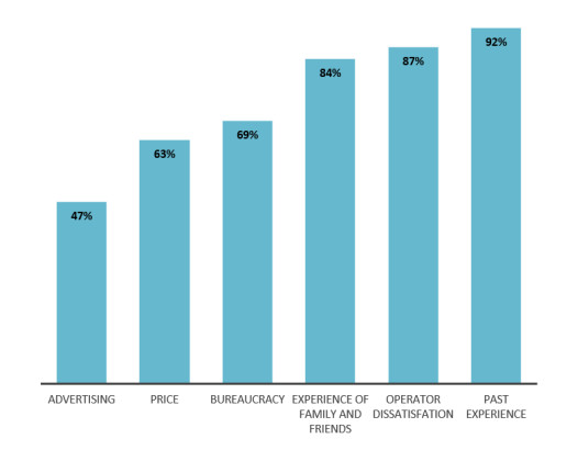
Electricity markets have been liberalized worldwide, but the success of country specific experiences varied widely. Consumers' behavior is among the key factors for successful liberalization experiences namely regarding the decision to switch operator. This decision has been shown to be influenced by a multiplicity of factors. The goal of this article is to explore the analysis of the drivers for switching operator in a liberalized electricity market. With that purpose, we focused on the residential Portuguese case using a questionnaire. The logit estimation showed that men are more likely to switch supplier than women and that larger families are less likely to do so probably, due to the perception of high information search costs. Other sociodemographic variables were not found to be statistically significant. Regarding specific determinants, our results showed that past experiences with a supplier, dissatisfaction with the current operator, and family and friends' experiences were the most important determining factor for the decision to switch operator. Hence, the price was not the most important determinant. We also explored if different income groups had differentiated responses regarding the main drivers but concluded that there was no evidence that the income group affected the importance given to the price or to the other determinants for the decision.
Citation: Débora Maravilha, Susana Silva, Erika Laranjeira. Consumer's behavior determinants after the electricity market liberalization: the Portuguese case[J]. Green Finance, 2022, 4(4): 436-449. doi: 10.3934/GF.2022021
Electricity markets have been liberalized worldwide, but the success of country specific experiences varied widely. Consumers' behavior is among the key factors for successful liberalization experiences namely regarding the decision to switch operator. This decision has been shown to be influenced by a multiplicity of factors. The goal of this article is to explore the analysis of the drivers for switching operator in a liberalized electricity market. With that purpose, we focused on the residential Portuguese case using a questionnaire. The logit estimation showed that men are more likely to switch supplier than women and that larger families are less likely to do so probably, due to the perception of high information search costs. Other sociodemographic variables were not found to be statistically significant. Regarding specific determinants, our results showed that past experiences with a supplier, dissatisfaction with the current operator, and family and friends' experiences were the most important determining factor for the decision to switch operator. Hence, the price was not the most important determinant. We also explored if different income groups had differentiated responses regarding the main drivers but concluded that there was no evidence that the income group affected the importance given to the price or to the other determinants for the decision.

| [1] |
Aliabadi DE, Chan K (2022) The emerging threat of artificial intelligence on competition in liberalized electricity markets: A deep Q-network approach. Appl Energy 32: 119813. https://doi.org/10.1016/j.apenergy.2022.119813 doi: 10.1016/j.apenergy.2022.119813

|
| [2] |
Al-Sunaidy A, Green R (2006) Electricity deregulation in OECD countries. Energy 31: 769–787. https://doi.org/10.1016/j.energy.2005.02.017 doi: 10.1016/j.energy.2005.02.017
|
| [3] | Ariu T, Lewis PE, Goto H, et al. (2012) Impacts and Lessons from the Fully Liberalized European Electricity Market - Residential Customer Price, Switching and Services. Central Research Institute of Electric Power Industry Report, No. Y11018. |
| [4] |
Armstrong M, Sappington D (2006) Regulation, Competition, and Liberalization. J Econ Lit 44: 325–366. https://doi.org/10.1257/jel.44.2.325 doi: 10.1257/jel.44.2.325
|
| [5] | Borenstein S, Bushnell J (2000) Electricity restructuring: deregulation or reregulation. Regulation 23: 46–52. |
| [6] |
Defeuilley C (2009) Retail competition in electricity markets. Energy Policy 37: 377–386. https://doi.org/10.1016/j.enpol.2008.07.025. doi: 10.1016/j.enpol.2008.07.025
|
| [7] | Drosos D, Grigorios LK, Arabatzis G, et al. (2020) Evaluating Customer Satisfaction in Energy Markets Using a Multicriteria Method: The Case of Electricity Market in Greece. Sustainability 12: 3862. https://doi.org/10.3390/su12093862 |
| [8] | ERSE (2013) Extinction of regulated tariffs for electricity and natural gas. Available from: http://www.erse.pt/eng/Paginas/extinctiontariffs.aspx. |
| [9] | ERSE (2021) Tarifas e preços para a energia elétrica e outros serviços em 2022 e parâmetros para o período de regulação 2022–2025. |
| [10] | ERSE (2021) Relatório sobre os mercados retalhistas de eletricidade e de gás natural em Portugal. |
| [11] | Entidade Reguladora dos Serviços Energético (ERSE) (2021) Síntese Mensal, November 2021. |
| [12] |
Ek K, Söderholm P (2008) Households' switching behavior between electricity suppliers in Sweden. Util Policy 16: 254–261. https://doi.org/10.1016/j.jup.2008.04.005. doi: 10.1016/j.jup.2008.04.005
|
| [13] |
Ferreira P, Araújo M, O'Kelly MEJ (2006) An overview of the portuguese electricity market. Energy Policy 35: 1967–1977. https://doi.org/10.1016/j.enpol.2006.06.003 doi: 10.1016/j.enpol.2006.06.003
|
| [14] | Flores M, Waddams PC (2013) Consumer behaviour in the British retail electricity market. Centre for Competition Policy Working Paper, University of East Anglia, Norwich (UK). https://ueaeco.github.io/working-papers/papers/ccp/CCP-13-10.pdf |
| [15] |
Gamble A, Juliusson E, Gärling T (2009) Consumer attitudes towards switching supplier in three deregulated markets. J Socio Econ 38: 814–819. https://doi.org/10.1016/j.socec.2009.05.002. doi: 10.1016/j.socec.2009.05.002
|
| [16] |
Gärling T, Gamble A, Juliusson E (2008) Consumers' switching inertia in a fictitious electricity market. Int J Consum Stud 32: 613–618. https://doi.org/10.1111/j.1470-6431.2008.00728.x doi: 10.1111/j.1470-6431.2008.00728.x
|
| [17] | Ghazvini M, Ramos S, Soares J, et al. (2019) Liberalization and customer behavior in the Portuguese residential retail electricity market. Util Policy 59: 100919. https://doi.org/10.1016/j.jup.2019.05.005 |
| [18] |
Giulietti M, Price C, Waterson M (2005) Consumer choice and competition policy: a study of UK energy markets. Econ J 115: 949–968. https://doi.org/10.1111/j.1468-0297.2005.01026.x doi: 10.1111/j.1468-0297.2005.01026.x
|
| [19] |
Hartmann P, Ibáñez VA (2007) Managing customer loyalty in liberalized residential energy markets: The impact of energy branding. Energy Policy 35: 2661–2672. https://doi.org/10.1016/j.enpol.2006.09.016 doi: 10.1016/j.enpol.2006.09.016
|
| [20] | Joskow PL (2011) Deregulation and regulatory reform. In Deregulation of Network Industries: What's Next? Sam Peltzman and Clifford Winston (Eds.). Washington D.C, USA, 113–188. |
| [21] |
Juliusson EA, Gamble A, Gärling T (2007) Loss aversion and price volatility as determinants of attitude towards variable price agreements in the Swedish electricity market. Energy Policy 35: 5953–5957. https://doi.org/10.1016/j.enpol.2007.06.019 doi: 10.1016/j.enpol.2007.06.019
|
| [22] |
Kaenzig J, Heinzle SL, Wüstenhagen R (2013) Whatever the customer wants, the customer gets? Exploring the gap between consumer preferences and default electricity products in Germany. Energy Policy 53: 311–322. https://doi.org/10.1016/j.enpol.2012.10.061 doi: 10.1016/j.enpol.2012.10.061
|
| [23] | Littlechild SC (2000) Why do we need electricity retailers: A reply to Joskow on wholesale spot price pass-through. University of Cambridge, Cambridge (UK). |
| [24] | Macedo DP, Marques AC, Damette O (2020) The impact of the integration of renewable energy sources in the electricity price formation: is the Merit-Order Effect occurring in Portugal? Util Policy 101080. https://doi.org/10.1016/j.jup.2020.101080 |
| [25] | Morey MJ, Kirsch LD (2016) Retail choice in electricity: What have we learned in 20 years? Electric Markets Research Foundation report. |
| [26] |
Pollitt M (2012) The role of policy in energy transitions: Lessons from the energy liberalisation era. Energy Policy 50: 128–137. https://doi.org/10.1016/j.enpol.2012.03.004 doi: 10.1016/j.enpol.2012.03.004
|
| [27] |
Roe B, Teisl M, Levy A, et al. (2001) US consumers' willingness to pay for green electricity. Energy policy 29: 917–925. https://doi.org/10.1016/S0301-4215(01)00006-4 doi: 10.1016/S0301-4215(01)00006-4
|
| [28] |
Shin KJ, Managi S (2017) Liberalization of a retail electricity market: Consumer satisfaction and household switching behavior in Japan. Energy Policy 110: 675–685. https://doi.org/10.1016/j.enpol.2017.07.048 doi: 10.1016/j.enpol.2017.07.048
|
| [29] | Sioshansi F (2006) Electricity Market Reform: What has the Experience taught us thus far? Util Policy 14: 63–75. https://doi.org/10.1016/j.jup.2005.12.002 |
| [30] |
Six M, Wirl F, Wolf J (2017) Information as potential key determinant in switching electricity suppliers. J Bus Econ 87: 263–290. https://doi.org/10.1007/s11573-016-0821-9 doi: 10.1007/s11573-016-0821-9
|
| [31] |
Vihalemm T, Keller M (2016) Consumers, citizens or citizen-consumers? Domestic users in the process of Estonian electricity market liberalization. Energy Res Soc Sci 13: 38–48. https://doi.org/10.1016/j.erss.2015.12.004 doi: 10.1016/j.erss.2015.12.004
|
| [32] |
Waterson M (2003) The role of consumer in competition and competition policy. Ind J Ind Organ 21: 129–150. https://doi.org/10.1016/S0167-7187(02)00054-1 doi: 10.1016/S0167-7187(02)00054-1
|
| [33] |
Woo CK, Lloyd D, Tishler A (2003) Electricity Market Reform Failures: UK, Norway, Alberta and California. Energy Policy 31: 1103–1115. https://doi.org/10.1016/S0301-4215(02)00211-2 doi: 10.1016/S0301-4215(02)00211-2
|
| [34] |
Yang Y (2014) Understanding household switching behavior in the retail electricity market. Energy Policy 69: 406–414. https://doi.org/10.1016/j.enpol.2014.03.009 doi: 10.1016/j.enpol.2014.03.009
|
Figures(1) / Tables(3)

Débora Maravilha, Susana Silva, Erika Laranjeira. Consumer's behavior determinants after the electricity market liberalization: the Portuguese case[J]. Green Finance, 2022, 4(4): 436-449. doi: 10.3934/GF.2022021


 DownLoad: