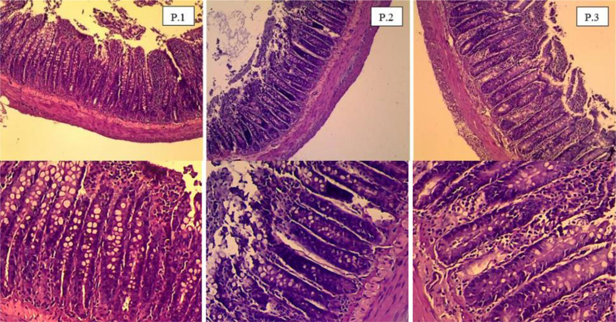
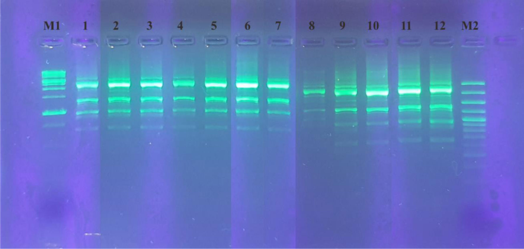
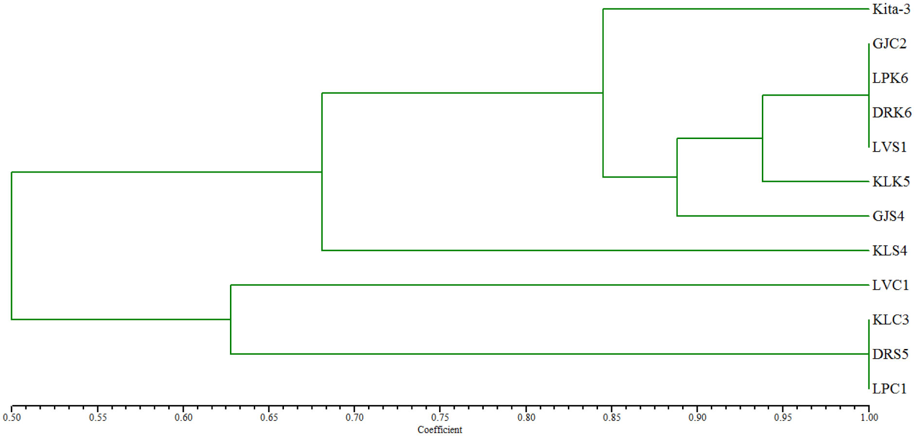
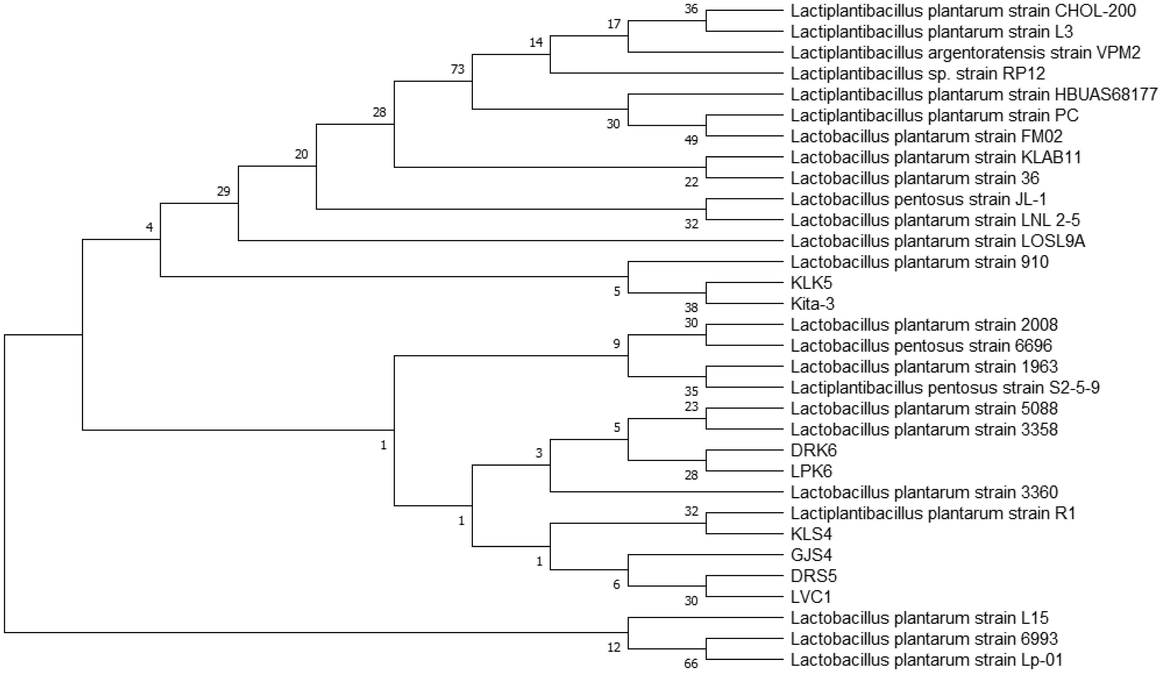
Lactiplantibacillus plantarum subsp. plantarum Kita-3 is a candidate probiotic from Halloumi cheese produced by Mazaraat Artisan Cheese, Yogyakarta, Indonesia. This study evaluated the safety of consuming a high dose of L. plantarum subsp. plantarum Kita-3 in Sprague-Dawley rats for 28 days. Eighteen male rats were randomly divided into three groups, such as the control group, the skim milk group, and the probiotic group. Feed intake and body weight were monitored, and blood samples, organs (kidneys, spleen, and liver), and the colon were dissected. Organ weight, hematological parameters, serum glutamic oxaloacetic transaminase (SGOT), and serum glutamic pyruvic transaminase (SGPT) concentrations, as well as intestinal morphology of the rats, were measured. Microbial analyses were carried out on the digesta, feces, blood, organs, and colon. The results showed that consumption of L. plantarum did not negatively affect general health, organ weight, hematological parameters, SGOT and SGPT activities, or intestinal morphology. The number of L. plantarum in the feces of rats increased significantly, indicating survival of the bacterium in the gastrointestinal tract. The bacteria in the blood, organs, and colon of all groups were identified using repetitive-polymerase chain reaction with the BOXA1R primers and further by 16S rRNA gene sequencing analysis, which revealed that they were not identical to L. plantarum subsp. plantarum Kita-3. Thus, this strain did not translocate to the blood or organs of rats. Therefore, L. plantarum subsp. plantarum Kita-3 is likely to be safe for human consumption.
Citation: Moh. A'inurrofiqin, Endang Sutriswati Rahayu, Dian Anggraini Suroto, Tyas Utami, Yunika Mayangsari. Safety assessment of the indigenous probiotic strain Lactiplantibacillus plantarum subsp. plantarum Kita-3 using Sprague–Dawley rats as a model[J]. AIMS Microbiology, 2022, 8(4): 403-421. doi: 10.3934/microbiol.2022028
Lactiplantibacillus plantarum subsp. plantarum Kita-3 is a candidate probiotic from Halloumi cheese produced by Mazaraat Artisan Cheese, Yogyakarta, Indonesia. This study evaluated the safety of consuming a high dose of L. plantarum subsp. plantarum Kita-3 in Sprague-Dawley rats for 28 days. Eighteen male rats were randomly divided into three groups, such as the control group, the skim milk group, and the probiotic group. Feed intake and body weight were monitored, and blood samples, organs (kidneys, spleen, and liver), and the colon were dissected. Organ weight, hematological parameters, serum glutamic oxaloacetic transaminase (SGOT), and serum glutamic pyruvic transaminase (SGPT) concentrations, as well as intestinal morphology of the rats, were measured. Microbial analyses were carried out on the digesta, feces, blood, organs, and colon. The results showed that consumption of L. plantarum did not negatively affect general health, organ weight, hematological parameters, SGOT and SGPT activities, or intestinal morphology. The number of L. plantarum in the feces of rats increased significantly, indicating survival of the bacterium in the gastrointestinal tract. The bacteria in the blood, organs, and colon of all groups were identified using repetitive-polymerase chain reaction with the BOXA1R primers and further by 16S rRNA gene sequencing analysis, which revealed that they were not identical to L. plantarum subsp. plantarum Kita-3. Thus, this strain did not translocate to the blood or organs of rats. Therefore, L. plantarum subsp. plantarum Kita-3 is likely to be safe for human consumption.

| [1] | FAO/WHOGuidelines for the evaluation of probiotics in food, London Ontario, Canada: report of a Joint FAO/WHO working for group on drafting guidelines for the evaluation of probiotics in food (2002). |
| [2] |
Holzapfel WH, Haberer P, Geisen R, et al. (2001) Taxonomy and important features of probiotic microorganisms in food and nutrition. Am J Clin Nutr 73: 365S-373S. https://doi.org/10.1093/ajcn/73.2.365s 
|
| [3] | Donohue DC (2006) Safety of probiotics. Asia Pac J Clin Nutr 15: 563-569. https://doi.org/10.1159/000345744 |
| [4] |
Kechagia M, Basoulis D, Konstantopoulou S, et al. (2013) Health benefits of probiotics: A review. ISRN Nutr 2013: 481651. https://doi.org/10.5402/2013/481651
|
| [5] | Rahayu ES (2003) Lactic acid bacteria in fermented foods of Indonesian origin. Agritech 23: 75-84. https://doi.org/10.22146/agritech.13515 |
| [6] |
Ratna DK, Evita MM, Rahayu ES, et al. (2021) Indigenous lactic acid bacteria from Halloumi cheese as a probiotics candidate of Indonesian origin. Int J Probiotics Prebiotics 16: 39-44. https://doi.org/10.37290/ijpp2641-7197.16:39-44
|
| [7] |
Gharaei-Fa E, Eslamifar M (2011) Isolation and applications of one strain of Lactobacillus paraplantarum from tea leaves (Camellia sinensis). Am J Food Technol 6: 429-434. https://doi.org/10.3923/ajft.2011.429.434
|
| [8] |
Kemgang TS, Kapila S, Shanmugam VP, et al. (2014) Cross-talk between probiotic Lactobacilli and host immune system. J Appl Microbiol 117: 303-319. https://doi.org/10.1111/jam.12521
|
| [9] |
Salminen S, von Wright A, Morelli L, et al. (1998) Demonstration of safety of probiotics: a review. Int J Food Microbiol 44: 93-106. https://doi.org/10.1016/S0168-1605(98)00128-7
|
| [10] |
Salminen MK, Rautelin H, Tynkkynen S, et al. (2006) Lactobacillus bacteremia, species identification, and antimicrobial susceptibility of 85 blood isolates. Clin Infect Dis 42: e35-e44. https://doi.org/10.1086/500214
|
| [11] |
Rahayu ES, Rusdan IH, Athennia A, et al. (2019) Safety assessment of indigenous probiotic strain Lactobacillus plantarum Dad-13 isolated from dadih using Sprague-Dawley rats as a model. Am J Pharmacol Toxicol 14: 38-47. https://doi.org/10.3844/ajptsp.2019.38.47
|
| [12] | Rinanda T (2011) 16S rRNA sequencing analysis in microbiology. Syiah Kuala Med J 11: 172-177. |
| [13] |
Ventura M, Zink R (2002) Specific identification and molecular typing analysis of Lactobacillus johnsonii by using PCR-based methods and pulsed-field gel electrophoresis. FEMS Microbiol Lett 217: 141-154. https://doi.org/10.1111/j.1574-6968.2002.tb11468.x
|
| [14] |
Ikhsani AY, Riftyan E, Safitri RA, et al. (2020) Safety assessment of indigenous probiotic strain Lactobacillus plantarum Mut-7 using Sprague–Dawley rats as a model. Am J Pharmacol Toxicol 15: 7-16. https://doi.org/10.3844/ajptsp.2020.7.16
|
| [15] |
Stackebrandt E, Goebel BM (1994) Taxonomic note: a place for DNA-DNA reassociation and 16S rRNA sequence analysis in the present species definition in bacteriology. Int J Syst Evol Microbiol 44: 846-849. https://doi.org/10.1099/00207713-44-4-846
|
| [16] |
Reeves PG, Nielsen FH, Fahey GC (1993) AIN-93 purified diets for laboratory rodents: final report of the American Institute of Nutrition Ad Hoc Writing Committee on the Reformulation of the AIN-76A Rodent Diet. J Nutr 123: 1939-1951. https://doi.org/10.1093/jn/123.11.1939
|
| [17] |
Shu Q, Zhou JS, J. Rutherfurd KJ, et al. (1999) Probiotic lactic acid bacteria (Lactobacillus acidophilus HN017, Lactobacillus rhamnosus HN001 and Bifidobacterium lactis HN019) have no adverse effects on the health of mice. Int Dairy J 9: 831-836. https://doi.org/10.1016/S0958-6946(99)00154-5
|
| [18] |
Zhou JS, Shu Q, Rutherfurd KJ, et al. (2000) Acute oral toxicity and bacterial translocation studies on potentially probiotic strains of lactic acid bacteria. Food Chem Toxicol 38: 153-161. https://doi.org/10.1016/S0278-6915(99)00154-4
|
| [19] |
Steppe M, Nieuwerburgh FV, Vercauteren G, et al. (2014) Safety assessment of the butyrate-producing Butyricicoccus pullicaecorum strain 25–3T, a potential probiotic for patients with inflammatory bowel disease, based on oral toxicity tests and whole genome sequencing. Food Chem Toxicol 72: 129-137. https://doi.org/10.1016/j.fct.2014.06.024
|
| [20] |
Zhou JS, Shu Q, Rutherfurd KJ, et al. (2000) Safety assessment of potential probiotic lactic acid bacterial strains Lactobacillus rhamnosus HN001, Lb. acidophilus HN017, and Bifidobacterium lactis HN019 in BALB/c mice. Int J Food Microbiol 56: 87-96. https://doi.org/10.1016/S0168-1605(00)00219-1
|
| [21] |
Bujalance C, Jiménez-Valera M, Moreno E, et al. (2006) A selective differential medium for Lactobacillus plantarum. J Microbiol Methods 66: 572-575. https://doi.org/10.1016/j.mimet.2006.02.005
|
| [22] |
Saxami G, Ypsilantis P, Sidira M, et al. (2012) Distinct adhesion of probiotic strain Lactobacillus casei ATCC 393 to rat intestinal mucosa. Anaerobe 18: 417-420. https://doi.org/10.1016/j.anaerobe.2012.04.002
|
| [23] |
Ismail YS, Yulvizar C, Mazhitov B (2018) Characterization of lactic acid bacteria from local cow's milk kefir. IOP Conference Series: Earth Environ Sci 130. https://doi.org/10.1088/1755-1315/130/1/012019
|
| [24] | (2022) Geneaid BiotechPresto™ mini gDNA bacteria kit protocol: instruction manual, ver. 02.10.17. New Taipei City, Taiwan: Geneaid Biotech Ltd. |
| [25] |
de Bruijn FJ (1992) Use of repetitive (repetitive extragenic palindromic and enterobacterial repetitive intergeneric consensus) sequences and the polymerase chain reaction to fingerprint the genomes of Rhizobium meliloti isolates and other soil bacteria. Appl Environ Microbiol 58: 2180-2187. https://doi.org/10.1128/aem.58.7.2180-2187.1992
|
| [26] |
Tamura K, Peterson D, Peterson N, et al. (2011) MEGA5: molecular evolutionary genetics analysis using maximum likelihood, evolutionary distance, and maximum parsimony methods. Mol Biol Evol 28: 2731-2739. https://doi.org/10.1093/molbev/msr121
|
| [27] | Spector WG (1977) An introduction to general pathology. London, UK: Churchill Livingstone. |
| [28] |
Kinnebrew MA, Pamer EG (2012) Innate immune signaling in defense against intestinal microbes. Immunol Rev 245: 113-131. https://doi.org/10.1111/j.1600-065X.2011.01081.x
|
| [29] |
Sanders ME, Akkermans LM, Haller D, et al. (2010) Safety assessment of probiotics for human use. Gut Microbes 1: 164-185. https://doi.org/10.4161/gmic.1.3.12127
|
| [30] |
Lara-Villoslada F, Sierra S, Díaz-Ropero MP, et al. (2009) Safety assessment of Lactobacillus fermentum CECT5716, a probiotic strain isolated from human milk. J Dairy Res 76: 216-221. https://doi.org/10.1017/S0022029909004014
|
| [31] |
Oyetayo VO, Adetuyi FC, Akinyosoye FA (2003) Safety and protective effect of Lactobacillus acidophilus and Lactobacillus casei used as probiotic agent in vivo. Afr J Biotechnol 2: 448-452. https://doi.org/10.5897/AJB2003.000-1090
|
| [32] | Takeuchi A, Sprinz H (1967) Electron-microscope studies of experimental Salmonella infection in the preconditioned guinea pig: II. Response of the intestinal mucosa to the invasion by Salmonella typhimurium. Am J Pathol 51: 137-161. |
| [33] |
Koch S, Nusrat A (2012) The life and death of epithelia during inflammation: lessons learned from the gut. Annu Rev Pathol 7: 35-60. https://doi.org/10.1146/annurev-pathol-011811-120905
|
| [34] |
Soderholm JD, Perdue MH (2006) Effect of stress on intestinal mucosal functions. Physiology of the gastrointestinal tract Burlington . San Diego and London: Elsevier Academic Press 763-780. https://doi.org/10.1016/B978-012088394-3/50031-3
|
| [35] |
Nagpal R, Yadav H (2017) Bacterial translocation from the gut to the distant organs: an overview. Ann Nutr Metab 71 Supplement 1: 11-16. https://doi.org/10.1159/000479918
|
| [36] |
Kechagia M, Basoulis D, Konstantopoulou S, et al. (2013) Health benefits of probiotics: a review. ISRN Nutr 2013: 481651. http://doi.org/10.5402/2013/481651
|
| [37] |
Sekirov I, Russell SL, Antunes LCM, et al. (2010) Gut microbiota in health and disease. Physiol Rev 90: 859-904. https://doi.org/10.1152/physrev.00045.2009
|
| [38] |
Trevisi P, de Filippi S, Modesto M, et al. (2007) Investigation on the ability of different strains and doses of exogenous Bifidobacteria, to translocate in the liver of weaning pigs. Livest Sci 108: 109-112. https://doi.org/10.1016/j.livsci.2007.01.007
|
| [39] |
Vastano V, Capri U, Candela M, et al. (2013) Identification of binding sites of Lactobacillus plantarum enolase involved in the interaction with human plasminogen. Microbiol Res 168: 65-72. https://doi.org/10.1016/j.micres.2012.10.001
|
| [40] |
Schillinger U, Lücke FK (1987) Identification of Lactobacilli from meat and meat products. Food Microbiol 4: 199-208. https://doi.org/10.1016/0740-0020(87)90002-5
|
| [41] | Holt JG, Krieg NL, Sneath PHA, et al. (1994) Bergey's manual of determinative bacteriology. Maryland, USA: Williams & Wilkins. |
| [42] |
Lee G (2013) Ciprofloxacin resistance in Enterococcus faecalis strains isolated from male patients with complicated urinary tract infection. Korean J Urol 54: 388-393. https://doi.org/10.4111/kju.2013.54.6.388
|
| [43] |
Masco L, Huys G, Gevers D, et al. (2003) Identification of Bifidobacterium species using rep-PCR fingerprinting. Syst Appl Microbiol 26: 557-563. https://doi.org/10.1078/072320203770865864
|
| [44] |
Gevers D, Huys G, Swings J (2001) Applicability of rep-PCR fingerprinting for identification of Lactobacillus species. FEMS Microbiol Lett 205: 31-36. https://doi.org/10.1111/j.1574-6968.2001.tb10921.x
|
| [45] | Versalovic J, Schneider M, de Bruijn FJ, et al. (1994) Genomic fingerprinting of bacteria using repetitive sequence-based polymerase chain reaction. Methods Mol Cell Biol 5: 25-40. |
| [46] |
Nucera DM, Lomonaco S, Costa A, et al. (2013) Diagnostic performance of rep-PCR as a rapid subtyping method for Listeria monocytogenes. Food Anal Methods 6: 868-871. https://doi.org/10.1007/s12161-012-9496-1
|
Figures(4) / Tables(7)

Moh. A'inurrofiqin, Endang Sutriswati Rahayu, Dian Anggraini Suroto, Tyas Utami, Yunika Mayangsari. Safety assessment of the indigenous probiotic strain Lactiplantibacillus plantarum subsp. plantarum Kita-3 using Sprague–Dawley rats as a model[J]. AIMS Microbiology, 2022, 8(4): 403-421. doi: 10.3934/microbiol.2022028


 DownLoad: